Azimuthal Averaging of Stellar Intensity#

Background#

The stellar intensity map from a YIP has real azimuthal structure, even for radially symmetric (1d) coronagraphs. Airy rings and diffraction features produce 70-90% azimuthal variation at moderate separations (e.g. r=10 pixels).

For yield calculations and integration time estimation, the azimuthally averaged stellar intensity at a given separation is typically desired rather than the raw position-angle-dependent value. This ensures that a planet’s background noise estimate depends only on its angular separation, not its arbitrary position angle.

Two Approaches#

Rotate-and-average (pyEDITH legacy)#

Rotate the 2D stellar intensity image through many angles and average:

from scipy.ndimage import rotate
import numpy as np

ntheta = 100
theta = np.linspace(0, 360, ntheta, endpoint=False)
result = np.zeros_like(istar_2d)
for angle in theta:
    result += rotate(istar_2d, angle, reshape=False, order=3)
result /= ntheta

This is conceptually simple but has several drawbacks:

Slow: 100 cubic interpolation passes (~0.4s per coronagraph)
Rotation artifacts: each scipy.ndimage.rotate call introduces cubic interpolation error that accumulates across rotations
Residual azimuthal structure: the averaged result is not perfectly symmetric, so the value at (r, PA=45deg) differs from (r, PA=47deg)

Radial profile projection (yippy)#

Bin pixels by radius, compute the mean in each annular bin, fit a 1D interpolator, and project back onto the pixel grid:

from yippy import Coronagraph

coro = Coronagraph(yip_path, psf_trunc_ratio=0.3)

# Already available: coro.core_mean_intensity(separation)
# To get a 2D map:
r_lod = coro.separation_map()  # (npix, npix) separations in lam/D
istar_az_avg = coro.core_mean_intensity(r_lod)

This approach:

Fast: a single vectorized interpolation call (~0.001s)
Artifact-free: no rotation interpolation artifacts
True azimuthal mean: mathematically exact average over all position angles, by definition
Perfectly symmetric: every pixel at the same radius gets the exact same value

Comparison#

Tested on usort_offaxis_ovc and eac1_aavc coronagraphs (256x256, pixscale=0.25 lam/D), comparing within 32 lam/D:

Metric	usort	eac1
Rotate time (100 angles)	0.424s	0.422s
Radial profile time	0.001s	0.001s
Speedup	365x	424x
Max relative difference	1288% (1e-17 center)	109%
Mean relative difference	3.0%	3.4%

The large max relative differences occur at near-zero-signal pixels close to the center where relative percentages blow up. The mean ~3% difference is real and originates from rotation interpolation artifacts in the rotate-and-average method.

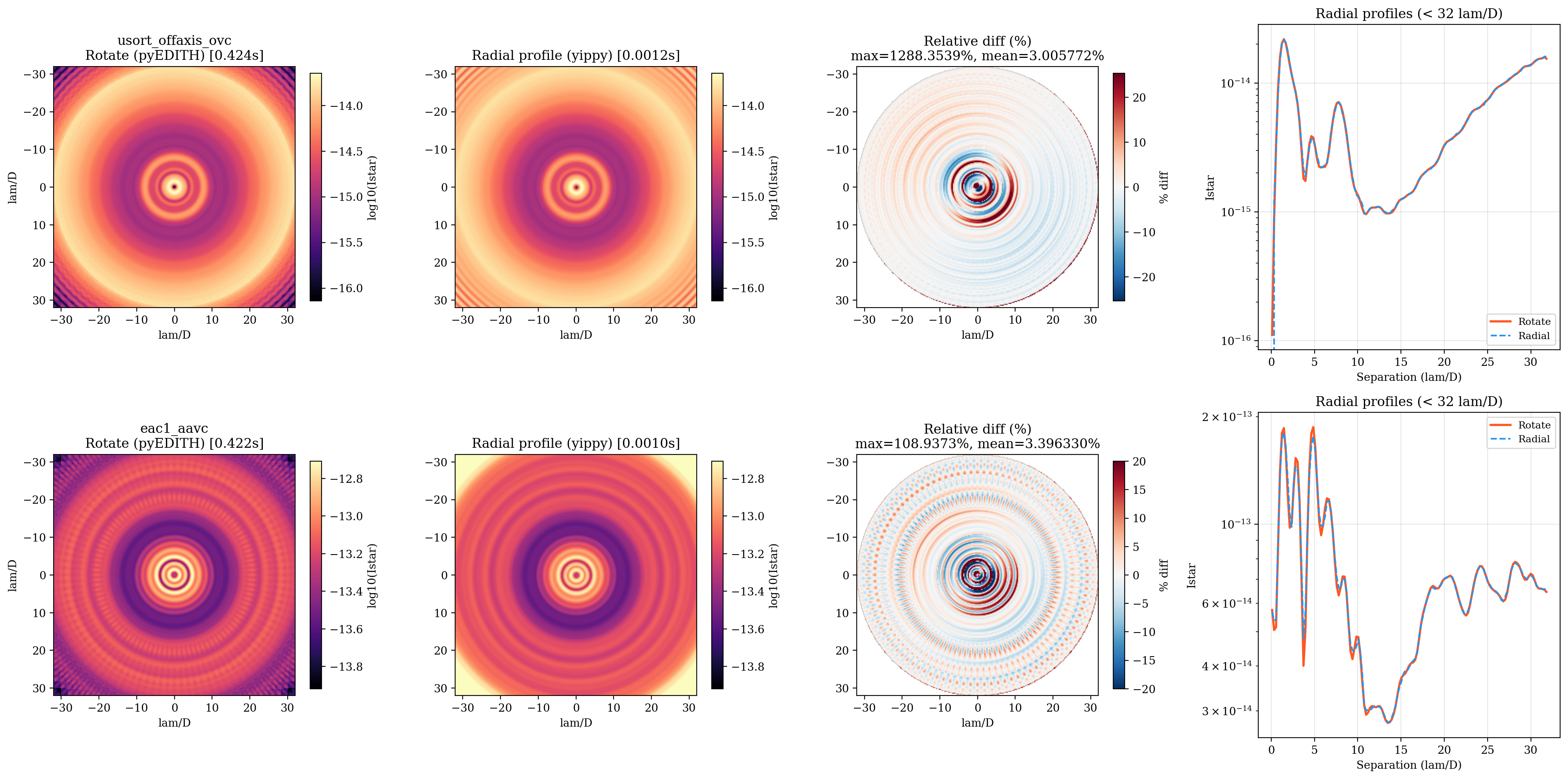
Comparison of rotate vs radial profile azimuthal averaging

Left pair: 2D maps (log scale) from each method appear visually similar, with clear Airy ring structure. Third column: relative difference map reveals systematic ring-pattern offsets at Airy ring peaks/troughs. Right: radial profiles overlay, showing the radial profile method (blue dashed) produces a smoother curve than the rotate method (orange solid).

Radial Binning Parameters#

The radial profile uses floor(max(image_shape) / 2) bins (128 for a 256x256 image). Each bin spans ~1.4 pixels (~0.35 lam/D at pixscale=0.25), giving ~3 bins per Airy ring spacing. This is adequate for capturing the azimuthal average without tracking fine Airy ring oscillations, which is desirable for the averaged quantity.

Recommendation#

Use yippy’s core_mean_intensity (radial profile) instead of the rotate-and-average approach. It is faster, more accurate, and produces cleaner azimuthal averages.

For the noise floor, divide by the post-processing factor:

noise_floor_ayo = coro.core_mean_intensity(separation) / ppf

Azimuthal Averaging of Stellar Intensity

Contents