Performance Metrics Overview

Coronagraph performance metrics bridge the gap between optical design and predicted scientific yield, ultimately determining the integration time required to detect or characterize an exoplanet.

This notebook provides a high-level dashboard of yippy’s performance metrics and shows how they feed into exposure time calculators (ETCs). For detailed theory and calculations, see the individual deep-dive notebooks:

• Core Throughput – planet signal preservation

• Stellar Leakage and Contrast – starlight suppression

• Spatial Metrics and Backgrounds – PSF core size and background scaling

• Noise Floors and Integration Time – systematic limits and ETC equations

Reference: Ruane et al. (2018) – Review of high-contrast imaging systems for current and future ground- and space-based telescopes I: coronagraph design methods and optical performance metrics

Reference: Stark et al. (2025) – Cross-Model Validation of Coronagraphic ExposureConfig Time Calculators for the Habitable Worlds Observatory

EXOSIMS utility: EXOSIMS provides its own YIP processing script, process_opticalsys_package, which computes throughput, core area, occulter transmission, and core mean intensity from the same input files that yippy reads.

---

Acknowledgments

Thank you to Susan Redmond for providing the AAVC coronagraph yield input package used throughout these demonstrations

Two ETC Families

Two primary exposure time calculators consume yippy’s coronagraph data, and they use fundamentally different aperture strategies:

	EXOSIMS	AYO / pyEDITH
Aperture	Fixed circular (e.g., 0.7 \(\lambda/D\))	PSF truncation ratio (adaptive)
Core Area	Constant	Varies with separation
Stellar leakage	Core Mean Intensity or Raw Contrast (fallback)	Core Mean Intensity
Noise floor	Contrast units	Intensity units
Background factor	1x (Nemati: RDI \(k_{SZ}\), \(k_{det}\))	2x (ADI subtraction)

Metrics at a Glance

Metric	yippy accessor	Description	Units
Core Throughput	coro.throughput(r)	Fraction of planet flux inside photometric aperture	dimensionless
Raw Contrast	coro.raw_contrast(r)	Stellar leakage relative to peak planet flux in aperture	dimensionless
Occulter Transmission	coro.occulter_transmission(r)	Sky transmission mask radial profile	dimensionless
Core Area	coro.core_area(r)	Effective solid angle of the PSF core	\((\lambda/D)^2\)
Core Mean Intensity	coro.core_mean_intensity(r)	Azimuthally averaged stellar intensity at separation \(r\)	dimensionless
Noise Floor (EXOSIMS)	coro.noise_floor_exosims(r)	\(\max(|C(r)|,\, C_{\rm floor}) / \text{ppf}\)	dimensionless
Noise Floor (AYO)	coro.noise_floor_ayo(r)	\(\bar{I}_\star(r) / \text{ppf}\)	dimensionless

Show code cell source

Hide code cell source

import matplotlib.pyplot as plt
import numpy as np
from yippy import fetch_yip
from yippy import Coronagraph

import logging; logging.getLogger("yippy").setLevel(logging.ERROR)

yip_path = fetch_yip("eac1_aavc_2d")
coro = Coronagraph(yip_path)
print(f"Coronagraph: {coro.name} (Amplitude Apodized Vortex Coronagraph, generated by Susan Redmond)")
print(f"IWA: {coro.IWA:.2f}")
print(f"OWA: {coro.OWA:.2f}")

/home/docs/checkouts/readthedocs.org/user_builds/yippy/envs/latest/lib/python3.12/site-packages/tqdm/auto.py:21: TqdmWarning: IProgress not found. Please update jupyter and ipywidgets. See https://ipywidgets.readthedocs.io/en/stable/user_install.html
  from .autonotebook import tqdm as notebook_tqdm

Downloading file 'eac1_aavc_2d.zip' from 'https://github.com/CoreySpohn/yippy/releases/download/data-v2/eac1_aavc_2d.zip' to '/home/docs/.cache/yippy'.

Unzipping contents of '/home/docs/.cache/yippy/eac1_aavc_2d.zip' to '/home/docs/.cache/yippy/eac1_aavc_2d.zip.unzip'

Coronagraph: eac1_aavc_2d (Amplitude Apodized Vortex Coronagraph, generated by Susan Redmond)
IWA: 4.26 λ/D
OWA: 32.00 λ/D

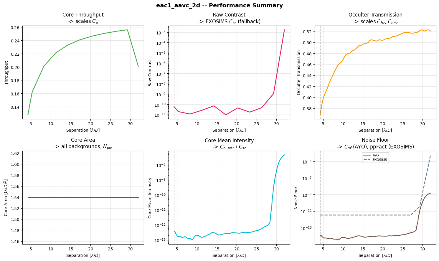
Summary Panel

Show code cell source

Hide code cell source

seps = np.linspace(coro.IWA.value, coro.OWA.value, 200)

fig, axes = plt.subplots(2, 3, figsize=(15, 9))

ax = axes[0, 0]
ax.plot(seps, coro.throughput(seps), color='#4CAF50', lw=2)
ax.set_ylabel('Throughput')
ax.set_title('Core Throughput\n-> scales $C_p$')
ax.grid(True, alpha=0.3)

ax = axes[0, 1]
ax.semilogy(seps, coro.raw_contrast(seps), color='#E91E63', lw=2)
ax.set_ylabel('Raw Contrast')
ax.set_title('Raw Contrast\n-> EXOSIMS $C_{sr}$ (fallback)')
ax.grid(True, alpha=0.3)

ax = axes[0, 2]
ax.plot(seps, coro.occulter_transmission(seps), color='#FF9800', lw=2)
ax.set_ylabel('Occulter Transmission')
ax.set_title('Occulter Transmission\n-> scales $C_{bz}$, $C_{bez}$')
ax.grid(True, alpha=0.3)

ax = axes[1, 0]
ax.plot(seps, coro.core_area(seps), color='#9C27B0', lw=2)
ax.set_ylabel('Core Area [$(\\lambda/D)^2$]')
ax.set_title('Core Area\n-> all backgrounds, $N_{pix}$')
ax.grid(True, alpha=0.3)

ax = axes[1, 1]
ax.semilogy(seps, coro.core_mean_intensity(seps), color='#00BCD4', lw=2)
ax.set_ylabel('Core Mean Intensity')
ax.set_title('Core Mean Intensity\n-> $C_{b,star}$ / $C_{sr}$')
ax.grid(True, alpha=0.3)

ax = axes[1, 2]
ax.semilogy(seps, coro.noise_floor_ayo(seps), color='#795548', lw=2,
            label='AYO')
ax.semilogy(seps, coro.noise_floor_exosims(seps), color='#607D8B',
            lw=2, ls='--', label='EXOSIMS')
ax.set_ylabel('Noise Floor')
ax.set_title('Noise Floor\n-> $C_{nf}$ (AYO), ppFact (EXOSIMS)')
ax.legend(fontsize=8)
ax.grid(True, alpha=0.3)

for ax in axes.flat:
    ax.set_xlabel('Separation [$\\lambda/D$]')
    ax.axvline(coro.IWA.value, ls='--', color='gray', alpha=0.5)

fig.suptitle(f'{coro.name} -- Performance Summary',
             fontsize=14, fontweight='bold')
plt.tight_layout()
plt.show()

---

How Metrics Feed Into ETCs

EXOSIMS Integration Time

\[t_{\text{int}} = \frac{\bar{c}_p + \bar{c}_b}{\left(\frac{\bar{c}_p}{\text{SNR}}\right)^2 - \bar{c}_{sp}^2}\]

where \(\bar{c}_{sp} = \bar{c}_{sr} \cdot \text{ppFact} \cdot \text{stabilityFact}\) is the photon rate of the speckle residual that fundamentally cannot be subtracted. Uses the fixed circular aperture mode.

Nemati Module

The equation above describes EXOSIMS’s default OpticalSystem, where \(\bar{c}_b\) is a simple sum of noise terms. The Nemati optical system module adds reference differential imaging (RDI) factors \(k_{SZ}\) and \(k_{det}\) that scale speckle/zodi and detector backgrounds respectively, based on the fraction of time spent on a reference star (ref_Time) and the reference star’s brightness difference (ref_dMag). See EXOSIMS.OpticalSystem.Nemati for details.

AYO / pyEDITH Integration Time

\[t_{\text{int}} = \frac{C_p + 2\, C_b}{\left(\frac{C_p}{\text{SNR}}\right)^2 - C_{nf}^2}\]

where the factor of 2 accounts for ADI background subtraction. Uses the PSF truncation aperture mode.