Spatial Metrics and Backgrounds

This notebook covers the metrics that govern background noise contributions: core area and occulter transmission. The physical size of the PSF core dictates how much background noise enters the photometric aperture.

Theory

Core Area

The core area \(\Omega\), measured in \((\lambda/D)^2\), represents the effective solid angle of the PSF core. It enters the ETC in two ways:

1. Detector pixels: \(N_{\rm pix} = \Omega / \theta_{\rm det}^2\) gives the number of detector pixels subtended by the core

2. Background scaling: All extended-source backgrounds (zodiacal dust, exozodiacal dust, detector noise) scale with \(\Omega\)

For a fixed circular aperture, the core area is constant: \(\Omega = \pi r_{ap}^2\). For the PSF truncation ratio method, the mask shape adapts to the PSF at each separation, so \(\Omega\) varies.

Occulter Transmission

Coronagraphs also reject light from extended background sources such as zodiacal and exozodiacal dust. The occulter transmission is the radial profile of the sky_trans.fits mask. In the ETC, it directly scales the background count rates \(C_{bz}\) and \(C_{bez}\).

API: Use compute_occ_trans_curve() for the radial profile, or access the raw 2D map via coro.sky_trans().

from yippy.performance import compute_occ_trans_curve
seps, occ_trans = compute_occ_trans_curve(coro)
# Or access the 2D sky transmission map:
sky_map = coro.sky_trans()  # 2D array

Show code cell source

Hide code cell source

import matplotlib.pyplot as plt
import numpy as np
from matplotlib import animation
from IPython.display import HTML
from yippy import fetch_yip
from yippy import Coronagraph
from yippy.performance import (
    compute_core_area_curve,
    compute_occ_trans_curve,
    compute_truncation_core_area_curve,
    compute_truncation_throughput_curve,
    compute_throughput_curve,
    _iter_xaxis_positions,
    _oversample_psf,
    _threshold_mask,
)

import logging; logging.getLogger("yippy").setLevel(logging.ERROR)

yip_path = fetch_yip("eac1_aavc_2d")
coro = Coronagraph(yip_path)
print(f"Coronagraph: {coro.name} (Amplitude Apodized Vortex Coronagraph, generated by Susan Redmond)")
print(f"Pixel scale: {coro.pixel_scale_arcsec}")
print(f"IWA: {coro.IWA:.2f}, OWA: {coro.OWA:.2f}")

/home/docs/checkouts/readthedocs.org/user_builds/yippy/envs/latest/lib/python3.12/site-packages/tqdm/auto.py:21: TqdmWarning: IProgress not found. Please update jupyter and ipywidgets. See https://ipywidgets.readthedocs.io/en/stable/user_install.html
  from .autonotebook import tqdm as notebook_tqdm

Coronagraph: eac1_aavc_2d (Amplitude Apodized Vortex Coronagraph, generated by Susan Redmond)
Pixel scale: 0.25 λ/D / pix
IWA: 4.26 λ/D, OWA: 32.00 λ/D

---

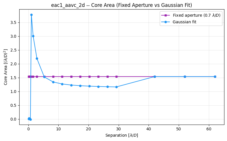
Core Area: Fixed Aperture

With a fixed circular aperture, core area is constant: \(\Omega = \pi r_{ap}^2\) in \((\lambda/D)^2\).

An alternative is to fit a 2D Gaussian to each PSF and compute \(\Omega = \pi \cdot \text{FWHM}_x \cdot \text{FWHM}_y / 4\) (shown below for comparison, but not typically used in ETCs).

API: Use compute_core_area_curve() for fixed apertures (with optional Gaussian fitting), or compute_truncation_core_area_curve() for truncation masks.

from yippy.performance import compute_core_area_curve, compute_truncation_core_area_curve
seps, areas = compute_core_area_curve(coro, aperture_radius_lod=0.7)
seps, areas = compute_truncation_core_area_curve(coro, psf_trunc_ratio=0.3)

Show code cell source

Hide code cell source

sep_a, area_fixed = compute_core_area_curve(
    coro, aperture_radius_lod=0.7, fit_gaussian=False
)
sep_g, area_gauss = compute_core_area_curve(
    coro, aperture_radius_lod=0.7, fit_gaussian=True
)

# Skip the first point where the Gaussian fit is unreliable
# (PSF at sep~0 is heavily suppressed, producing a bad fit)
fig, ax = plt.subplots(figsize=(8, 5))
ax.plot(sep_a[1:], area_fixed[1:], 's-', ms=5, color='#9C27B0',
        label='Fixed aperture (0.7 $\\lambda/D$)')
ax.plot(sep_g[1:], area_gauss[1:], 'o-', ms=5, color='#2196F3',
        label='Gaussian fit')
ax.set_xlabel('Separation [$\\lambda/D$]')
ax.set_ylabel('Core Area [$(\\lambda/D)^2$]')
ax.set_title(f'{coro.name} -- Core Area (Fixed Aperture vs Gaussian Fit)')
ax.legend()
ax.grid(True, alpha=0.3)
plt.tight_layout()
plt.show()

---

Core Area: Truncation Ratio Animation

With the PSF truncation ratio method, the core area varies with separation because the mask shape adapts to the PSF structure. The animation below shows the truncation mask (cyan contour) and the corresponding core area at each position, compared with the constant fixed-aperture value.

Show code cell source

Hide code cell source

from yippy.performance import _oversample_psf, _threshold_mask
from yippy.util import crop_around_peak

psf_trunc_ratio = 0.5
pix_lod = coro.pixel_scale_arcsec.value
os_factor = int(np.ceil(pix_lod / 0.05))
crop_radius = int(5 / (pix_lod / os_factor))  # +/-5 lam/D

positions = list(_iter_xaxis_positions(coro))

area_frames = []
for pos in positions:
    psf_os_full = _oversample_psf(pos.psf, pix_lod, os_factor)
    mask_full = _threshold_mask(psf_os_full, psf_trunc_ratio)
    n_pix = mask_full.sum()
    pix_to_fwhm = (pix_lod / os_factor) ** 2
    area_lod2 = n_pix * pix_to_fwhm
    # Crop both arrays centered on the PSF peak
    psf_os = crop_around_peak(psf_os_full, crop_radius)
    peak_y, peak_x = np.unravel_index(psf_os_full.argmax(), psf_os_full.shape)
    ny, nx = psf_os_full.shape
    r = min(crop_radius, peak_y, ny - peak_y, peak_x, nx - peak_x)
    mask = mask_full[peak_y - r:peak_y + r, peak_x - r:peak_x + r]
    area_frames.append({
        'sep': pos.separation,
        'full_psf': pos.psf,
        'psf_os': psf_os,
        'mask': mask,
        'area': area_lod2,
    })

# Compute global colorscale across all frames
global_peak_full = max(
    np.log10(np.maximum(f['full_psf'], 1e-20)).max() for f in area_frames
)
global_peak_mask = max(
    np.log10(np.maximum(f['psf_os'], 1e-20)).max() for f in area_frames
)

fig = plt.figure(figsize=(18, 5))
gs = fig.add_gridspec(1, 3, width_ratios=[1, 1, 1.2], wspace=0.3)
ax_full = fig.add_subplot(gs[0, 0])
ax_mask = fig.add_subplot(gs[0, 1])
ax_curve = fig.add_subplot(gs[0, 2])

# Full-frame PSF
f0 = area_frames[0]
log_full = np.log10(np.maximum(f0['full_psf'], 1e-20))

im_full = ax_full.imshow(log_full, origin='lower', cmap='magma',
                         vmin=global_peak_full - 5, vmax=global_peak_full)
ax_full.set_title('Off-axis PSF (full frame)')
ax_full.set_xlabel('x [pix]')
ax_full.set_ylabel('y [pix]')
ax_full.set_aspect('equal')

# Cropped oversampled PSF with mask
log_psf = np.log10(np.maximum(f0['psf_os'], 1e-20))

im = ax_mask.imshow(log_psf, origin='lower', cmap='magma',
                    vmin=global_peak_mask - 4, vmax=global_peak_mask)
contour_set = ax_mask.contour(f0['mask'].astype(float), levels=[0.5],
                             colors='cyan', linewidths=2)
ax_mask.set_title('Truncation mask (zoomed)')
ax_mask.set_xlabel('x [oversampled pix]')
ax_mask.set_aspect('equal')

title_fig = fig.suptitle('', fontsize=12)

# Core area curve
a_seps = [f['sep'] for f in area_frames]
a_vals = [f['area'] for f in area_frames]
ax_curve.plot(a_seps, a_vals, 'o-', ms=4, color='#CCCCCC', alpha=0.3, zorder=1)
scatter_a = ax_curve.scatter([], [], s=80, color='#9C27B0', zorder=3)
line_a, = ax_curve.plot([], [], 'o-', ms=5, color='#9C27B0', zorder=2)
ax_curve.axvline(coro.IWA.value, ls='--', color='gray', alpha=0.7,
                 label=f'IWA = {coro.IWA.value:.1f}')
ax_curve.set_xlabel('Separation [$\\lambda/D$]')
ax_curve.set_ylabel('Core Area [$(\\lambda/D)^2$]')
ax_curve.set_title(f'Core Area (ratio = {psf_trunc_ratio})')
ax_curve.legend()
ax_curve.grid(True, alpha=0.3)

def update_area(i):
    f = area_frames[i]

    # Update full-frame
    log_f = np.log10(np.maximum(f['full_psf'], 1e-20))
    im_full.set_data(log_f)

    # Update cropped mask view
    log_img = np.log10(np.maximum(f['psf_os'], 1e-20))
    im.set_data(log_img)
    im.set_extent([-0.5, log_img.shape[1]-0.5, -0.5, log_img.shape[0]-0.5])
    ax_mask.set_xlim(-0.5, log_img.shape[1]-0.5)
    ax_mask.set_ylim(-0.5, log_img.shape[0]-0.5)

    for coll in ax_mask.collections[:]:
        coll.remove()
    ax_mask.contour(f['mask'].astype(float), levels=[0.5],
                   colors='cyan', linewidths=2)

    title_fig.set_text(
        f"Sep = {f['sep']:.2f} $\\lambda/D$  |  "
        f"Core Area = {f['area']:.3f} $(\\lambda/D)^2$"
    )

    line_a.set_data(a_seps[:i+1], a_vals[:i+1])
    scatter_a.set_offsets([[f['sep'], f['area']]])
    return im_full, im, title_fig, line_a, scatter_a

anim = animation.FuncAnimation(fig, update_area, frames=len(area_frames),
                               interval=400, blit=False)
plt.close(fig)
HTML(anim.to_jshtml())

Once Loop Reflect

Fixed vs Truncation Comparison

Show code cell source

Hide code cell source

sep_f, tp_fixed = compute_throughput_curve(coro, aperture_radius_lod=0.7)
sep_af, area_f = compute_core_area_curve(coro, aperture_radius_lod=0.7)

sep_tr, tp_trunc = compute_truncation_throughput_curve(coro, psf_trunc_ratio=0.3)
sep_at, area_t = compute_truncation_core_area_curve(coro, psf_trunc_ratio=0.3)

fig, (ax1, ax2) = plt.subplots(1, 2, figsize=(14, 5))

ax1.plot(sep_f, tp_fixed, 'o-', ms=4, color='#4CAF50',
         label='Fixed aperture (0.7 $\\lambda/D$)')
ax1.plot(sep_tr, tp_trunc, 's-', ms=4, color='#FF5722',
         label='Truncation ratio (0.3)')
ax1.set_xlabel('Separation [$\\lambda/D$]')
ax1.set_ylabel('Throughput')
ax1.set_title('Throughput')
ax1.legend()
ax1.grid(True, alpha=0.3)

ax2.plot(sep_af, area_f, 'o-', ms=4, color='#9C27B0',
         label='Fixed aperture (0.7 $\\lambda/D$)')
ax2.plot(sep_at, area_t, 's-', ms=4, color='#FF5722',
         label='Truncation ratio (0.3)')
ax2.set_xlabel('Separation [$\\lambda/D$]')
ax2.set_ylabel('Core Area [$(\\lambda/D)^2$]')
ax2.set_title('Core Area')
ax2.legend()
ax2.grid(True, alpha=0.3)

fig.suptitle(f'{coro.name} -- Fixed Aperture vs PSF Truncation Ratio',
             fontsize=14, fontweight='bold')
plt.tight_layout()
plt.show()

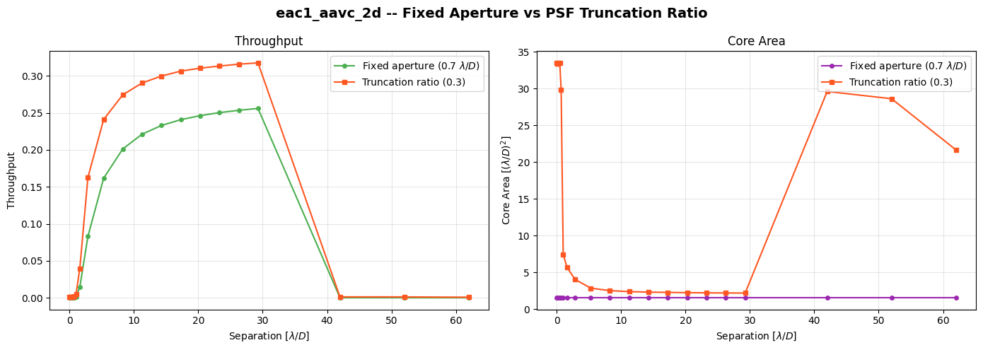
Note how the truncation-ratio core area varies with separation while the fixed aperture is constant. When calculating exposure times, AYO loops over multiple truncation ratios and picks the one that minimizes integration time at each separation.

For a deeper comparison of these two aperture methods, including noise metrics and AYO’s optimization strategy, see the Aperture Methods Comparison.

---

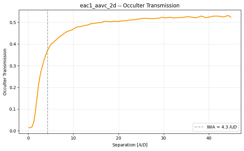
Occulter Transmission

Occulter transmission represents how much light from spatially extended background sources (zodiacal dust, exozodiacal dust) survives the coronagraph mask. It is the radial profile of the sky_trans.fits mask.

In the ETC, it scales all extended-source backgrounds (\(C_{bz}\), \(C_{bez}\)).

Show code cell source

Hide code cell source

sky_data = coro.sky_trans()
pix_scale = coro.pixel_scale_arcsec.value
owa_val = coro.OWA.value

# Center of the sky transmission map
cy_sky = sky_data.shape[0] / 2
cx_sky = sky_data.shape[1] / 2

# Compute the full radial profile
from hwoutils.radial import radial_profile
import jax.numpy as jnp

seps_ot, profile_ot = radial_profile(
    jnp.asarray(np.asarray(sky_data, dtype=np.float64)),
    pixel_scale_arcsec=pix_scale,
    nbins=int(np.floor(np.max(sky_data.shape) / 2)),
)
seps_ot = np.asarray(seps_ot)
profile_ot = np.asarray(profile_ot)

# Only show up to OWA
mask_owa = seps_ot <= owa_val * 1.1
step = max(1, len(seps_ot[mask_owa]) // 25)
frame_indices = list(range(0, len(seps_ot[mask_owa]), step))

fig_ot = plt.figure(figsize=(14, 5))
gs_ot = fig_ot.add_gridspec(1, 2, width_ratios=[1, 1.3], wspace=0.3)
ax_sky = fig_ot.add_subplot(gs_ot[0, 0])
ax_ot_prof = fig_ot.add_subplot(gs_ot[0, 1])

# Sky transmission image
im_sky = ax_sky.imshow(sky_data, origin='lower', cmap='magma',
                       vmin=0, vmax=1)
ax_sky.set_aspect('equal')
annulus_in = plt.Circle((cx_sky, cy_sky), 0, fill=False,
                        ec='white', lw=2)
annulus_out = plt.Circle((cx_sky, cy_sky), 0, fill=False,
                         ec='white', lw=2)
ax_sky.add_patch(annulus_in)
ax_sky.add_patch(annulus_out)
ax_sky.set_title('Sky Transmission Map')
ax_sky.set_xlabel('x [pix]')
ax_sky.set_ylabel('y [pix]')
plt.colorbar(im_sky, ax=ax_sky, shrink=0.8)

# Profile plot
ax_ot_prof.plot(seps_ot[mask_owa], profile_ot[mask_owa], '-',
                color='#CCCCCC', alpha=0.3, lw=2, zorder=1)
line_ot, = ax_ot_prof.plot([], [], '-', color='#4CAF50', lw=2, zorder=2)
dot_ot = ax_ot_prof.scatter([], [], s=80, color='#4CAF50', zorder=3)
ax_ot_prof.axvline(coro.IWA.value, ls='--', color='gray', alpha=0.7,
                   label=f'IWA = {coro.IWA.value:.1f}')
ax_ot_prof.axvline(owa_val, ls='--', color='gray', alpha=0.5,
                   label=f'OWA = {owa_val:.0f}')
ax_ot_prof.set_xlabel('Separation [$\\lambda/D$]')
ax_ot_prof.set_ylabel('Occulter Transmission')
ax_ot_prof.set_title('Radial Profile')
ax_ot_prof.set_ylim(-0.05, 1.05)
ax_ot_prof.set_xlim(0, owa_val * 1.1)
ax_ot_prof.legend()
ax_ot_prof.grid(True, alpha=0.3)

title_ot = fig_ot.suptitle('', fontsize=12)

def update_ot(frame_num):
    idx = frame_indices[frame_num]
    r_lod = seps_ot[idx]
    r_pix = r_lod / pix_scale
    dr_pix = (seps_ot[1] - seps_ot[0]) / pix_scale if idx > 0 else 1

    annulus_in.set_radius(max(0, r_pix - dr_pix))
    annulus_out.set_radius(r_pix + dr_pix)

    line_ot.set_data(seps_ot[:idx+1], profile_ot[:idx+1])
    dot_ot.set_offsets([[r_lod, profile_ot[idx]]])

    title_ot.set_text(
        f'Sep = {r_lod:.1f} $\\lambda/D$  |  '
        f'Transmission = {profile_ot[idx]:.3f}'
    )
    return annulus_in, annulus_out, line_ot, dot_ot, title_ot

anim_ot = animation.FuncAnimation(fig_ot, update_ot,
                                  frames=len(frame_indices),
                                  interval=200, blit=False)
plt.close(fig_ot)
HTML(anim_ot.to_jshtml())

Once Loop Reflect

Show code cell source

Hide code cell source

sep_ot, occ_trans = compute_occ_trans_curve(coro)

fig, ax = plt.subplots(figsize=(8, 5))
ax.plot(sep_ot, occ_trans, '-', color='#FF9800', lw=2)
ax.axvline(coro.IWA.value, ls='--', color='gray', alpha=0.7,
           label=f'IWA = {coro.IWA.value:.1f} $\\lambda/D$')
ax.set_xlabel('Separation [$\\lambda/D$]')
ax.set_ylabel('Occulter Transmission')
ax.set_title(f'{coro.name} -- Occulter Transmission')
ax.legend()
ax.grid(True, alpha=0.3)
plt.tight_layout()
plt.show()