Stellar Leakage and Contrast

This notebook covers the metrics that quantify how well the coronagraph suppresses the host star: raw contrast and core mean intensity. These determine the stellar leakage count rate in the ETC.

Theory

Raw Contrast

Raw contrast is the ratio of detected starlight to detected planet light:

\[C(x_0, \lambda) = \frac{\eta_s(x_0, \lambda)}{\eta_p(x_0, \lambda)}\]

Low contrast means the coronagraph effectively suppresses starlight.

Core Mean Intensity

An alternative is \(\bar{I}_\star(r)\), the azimuthally averaged stellar intensity at separation \(r\), used for per-pixel ETC calculations.

ETC Usage

ETC	Method	Formula
EXOSIMS (primary)	Core Mean Intensity	\(C_{sr} = C_\star \cdot \bar{I}_\star \cdot \Omega / \theta_{det}^2\)
EXOSIMS (fallback)	Raw Contrast	\(C_{sr} = C_\star \cdot C(r) \cdot \Upsilon_c(r)\)
AYO / pyEDITH	Core Mean Intensity	Per-pixel \(I_\star(x, y)\) map

API: Use compute_raw_contrast_curve() for the full curve, or access the interpolator via coro.raw_contrast(separation).

from yippy.performance import compute_raw_contrast_curve
seps, contrasts = compute_raw_contrast_curve(coro, aperture_radius_lod=0.7)
# Or use the interpolator:
C = coro.raw_contrast(8.0)  # raw contrast at 8 lam/D

API: Use compute_core_mean_intensity_curve() for the full radial profile per stellar diameter, or access the stored interpolator via coro.core_mean_intensity(separation, stellar_diam).

from yippy.performance import compute_core_mean_intensity_curve
seps, intensities = compute_core_mean_intensity_curve(coro)
# intensities is a dict: {stellar_diam: array}
# Or use the interpolator:
cmi = coro.core_mean_intensity(8.0, stellar_diam=0.0)  # at 8 lam/D, point source

Nomenclature: “Core Mean Intensity”

The name core mean intensity originates from EXOSIMS, where the radially averaged stellar intensity profile is stored as core_mean_intensity.fits (generated by process_opticalsys_package). Other tools use different names for the same quantity:

Tool	Variable Name	Description
EXOSIMS	core_mean_intensity	Radial average of stellar intensity map, stored as 1D curve
AYO	Istar	Raw 2D stellar intensity map (not radially averaged), indexed per pixel
pyEDITH	coronagraph.Istar	Same as AYO: raw 2D map from YIP
yippy	coro.core_mean_intensity()	Radial average, matching EXOSIMS convention

Despite the name, it is not computed within a photometric aperture (“core”). It is the azimuthal mean of the full 2D stellar intensity map at each separation. The “core” qualifier reflects how the value is used in the ETC (\(\bar{I}_\star \cdot \Omega\), where \(\Omega\) is the core area), not how it is computed.

Note that AYO and pyEDITH work directly with the 2D Istar map and look up the per-pixel value at the planet’s position, while EXOSIMS and yippy use the radially averaged 1D profile.

Show code cell source

Hide code cell source

import matplotlib.pyplot as plt
import numpy as np
from matplotlib.patches import Circle, Rectangle
from matplotlib import animation
from IPython.display import HTML
from lod_unit import lod
from yippy import fetch_yip
from yippy import Coronagraph
from yippy.performance import (
    compute_throughput_curve,
    compute_raw_contrast_curve,
    compute_core_mean_intensity_curve,
    _iter_xaxis_positions,
    _point_source_in_image,
)
from yippy.util import (
    extract_and_oversample_subarray,
    measure_flux_in_oversampled_aperture,
    crop_around_peak,
)
import logging; logging.getLogger("yippy").setLevel(logging.ERROR)

yip_path = fetch_yip("eac1_aavc_2d")
coro = Coronagraph(yip_path)
print(f"Coronagraph: {coro.name} (Amplitude Apodized Vortex Coronagraph, generated by Susan Redmond)")
print(f"IWA: {coro.IWA:.2f}, OWA: {coro.OWA:.2f}")

/home/docs/checkouts/readthedocs.org/user_builds/yippy/envs/latest/lib/python3.12/site-packages/tqdm/auto.py:21: TqdmWarning: IProgress not found. Please update jupyter and ipywidgets. See https://ipywidgets.readthedocs.io/en/stable/user_install.html
  from .autonotebook import tqdm as notebook_tqdm

Coronagraph: eac1_aavc_2d (Amplitude Apodized Vortex Coronagraph, generated by Susan Redmond)
IWA: 4.26 λ/D, OWA: 32.00 λ/D

---

Contrast Measurement Animation

Raw contrast requires measuring flux in the same aperture in both the off-axis (planet) PSF and the on-axis (stellar) PSF. The animation below shows the full-frame images (top), zoomed views around the photometric aperture (middle), and the contrast curve building up (bottom).

All images share the same color scale (set by the planet PSF peak) so you can visually see how much fainter the stellar leakage is – this difference is exactly the raw contrast.

Show code cell source

Hide code cell source

aperture_radius_lod = 0.7
oversample = 2
radius_pix = aperture_radius_lod / coro.pixel_scale_arcsec.value

star_psf = coro.stellar_intens(0.0 * lod)

positions = [p for p in _iter_xaxis_positions(coro) if _point_source_in_image(p)]

contrast_frames = []
for pos in positions:
    # Planet PSF zoom
    sub_p, px_p, py_p, r_p, orig_p = extract_and_oversample_subarray(
        pos.psf, pos.px, pos.py, radius_pix, oversample
    )
    peak_p = np.unravel_index(sub_p.argmax(), sub_p.shape)
    planet_flux = measure_flux_in_oversampled_aperture(
        sub_p, float(peak_p[1]), float(peak_p[0]), r_p, orig_p
    )
    # Star PSF zoom at the same position
    sub_s, px_s, py_s, r_s, orig_s = extract_and_oversample_subarray(
        star_psf, pos.px, pos.py, radius_pix, oversample
    )
    star_flux = measure_flux_in_oversampled_aperture(
        sub_s, px_s, py_s, r_s, orig_s
    )
    c_val = star_flux / planet_flux if planet_flux > 0 else np.inf
    contrast_frames.append({
        'sep': pos.separation,
        'full_planet': pos.psf,
        'full_star': star_psf,
        'px': pos.px, 'py': pos.py,
        'sub_p': sub_p, 'sub_s': sub_s,
        'cx_p': px_p, 'cy_p': py_p,
        'cx_s': px_s, 'cy_s': py_s,
        'r_p': r_p, 'r_s': r_s,
        'planet_flux': planet_flux,
        'star_flux': star_flux,
        'contrast': c_val,
    })

# 3-row x 2-col layout
# Compute global colorscale across all frames
global_planet_peak = max(
    np.log10(np.maximum(f['full_planet'], 1e-20)).max()
    for f in contrast_frames
)
global_zoom_peak = max(
    np.log10(np.maximum(f['sub_p'], 1e-20)).max()
    for f in contrast_frames
)

fig = plt.figure(figsize=(12, 14))
gs = fig.add_gridspec(3, 2, height_ratios=[1, 1, 0.8],
                      hspace=0.3, wspace=0.25)

# Row 0: full-frame images
ax_fp = fig.add_subplot(gs[0, 0])
ax_fs = fig.add_subplot(gs[0, 1])
# Row 1: zoomed views
ax_zp = fig.add_subplot(gs[1, 0])
ax_zs = fig.add_subplot(gs[1, 1])
# Row 2: contrast curve spanning both columns
ax_curve = fig.add_subplot(gs[2, :])

f0 = contrast_frames[0]

def log_img(arr):
    return np.log10(np.maximum(arr, 1e-20))

# Shared colorscale anchored to planet PSF peak (6 dex range)
log_p0 = log_img(f0['full_planet'])
shared_vmax = global_planet_peak
shared_vmin = global_planet_peak - 6

# -- Row 0: Full-frame planet and star --
im_fp = ax_fp.imshow(log_p0, origin='lower', cmap='magma',
                     vmin=shared_vmin, vmax=shared_vmax)
circ_fp = Circle((f0['px'], f0['py']), radius_pix,
                 fill=False, ec='cyan', lw=1.5, ls='--')
ax_fp.add_patch(circ_fp)
# Zoom indicator rectangle on full planet
zoom_half = radius_pix * 3  # same as extract_and_oversample margin
rect_fp = Rectangle((f0['px'] - zoom_half, f0['py'] - zoom_half),
                    2 * zoom_half, 2 * zoom_half,
                    fill=False, ec='white', lw=1, ls=':')
ax_fp.add_patch(rect_fp)
ax_fp.set_title('Planet PSF (full frame)')
ax_fp.set_xlabel('x [pix]')
ax_fp.set_ylabel('y [pix]')
ax_fp.set_aspect('equal')

log_s0 = log_img(f0['full_star'])
im_fs = ax_fs.imshow(log_s0, origin='lower', cmap='magma',
                     vmin=shared_vmin, vmax=shared_vmax)
circ_fs = Circle((f0['px'], f0['py']), radius_pix,
                 fill=False, ec='lime', lw=1.5, ls='--')
ax_fs.add_patch(circ_fs)
rect_fs = Rectangle((f0['px'] - zoom_half, f0['py'] - zoom_half),
                    2 * zoom_half, 2 * zoom_half,
                    fill=False, ec='white', lw=1, ls=':')
ax_fs.add_patch(rect_fs)
ax_fs.set_title('Star PSF (full frame, same scale)')
ax_fs.set_xlabel('x [pix]')
ax_fs.set_aspect('equal')

# Shared colorbar between the two full-frame panels
cbar = fig.colorbar(im_fp, ax=[ax_fp, ax_fs], location='right',
                    shrink=0.8, pad=0.02)
cbar.set_label('$\\log_{10}$(intensity)')

# -- Row 1: Zoomed planet and star (shared colorscale) --
log_zp0 = log_img(f0['sub_p'])
log_zs0 = log_img(f0['sub_s'])
zoom_vmax = global_zoom_peak
zoom_vmin = global_zoom_peak - 5

im_zp = ax_zp.imshow(log_zp0, origin='lower', cmap='magma',
                     vmin=zoom_vmin, vmax=zoom_vmax)
circ_zp = Circle((f0['cx_p'], f0['cy_p']), f0['r_p'],
                 fill=False, ec='cyan', lw=2, ls='--')
ax_zp.add_patch(circ_zp)
ax_zp.set_title('Planet PSF (zoomed)')
ax_zp.set_xlabel('x [oversampled pix]')
ax_zp.set_ylabel('y [oversampled pix]')
ax_zp.set_aspect('equal')

im_zs = ax_zs.imshow(log_zs0, origin='lower', cmap='magma',
                     vmin=zoom_vmin, vmax=zoom_vmax)
circ_zs = Circle((f0['cx_s'], f0['cy_s']), f0['r_s'],
                 fill=False, ec='lime', lw=2, ls='--')
ax_zs.add_patch(circ_zs)
ax_zs.set_title('Star PSF (zoomed, same scale)')
ax_zs.set_xlabel('x [oversampled pix]')
ax_zs.set_aspect('equal')

cbar_zoom = fig.colorbar(im_zp, ax=[ax_zp, ax_zs], location='right',
                         shrink=0.8, pad=0.02)
cbar_zoom.set_label('$\\log_{10}$(intensity)')

title_fig = fig.suptitle('', fontsize=13, y=0.98)

# -- Row 2: Contrast curve --
c_seps = [f['sep'] for f in contrast_frames]
c_vals = [f['contrast'] for f in contrast_frames]
ax_curve.semilogy(c_seps, c_vals, 'o-', ms=4, color='#CCCCCC',
                  alpha=0.3, zorder=1)
scatter_c = ax_curve.scatter([], [], s=80, color='#E91E63', zorder=3)
line_c, = ax_curve.plot([], [], 'o-', ms=5, color='#E91E63', zorder=2)
ax_curve.axvline(coro.IWA.value, ls='--', color='gray', alpha=0.7,
                 label=f'IWA = {coro.IWA.value:.1f}')
ax_curve.set_xlabel('Separation [$\\lambda/D$]')
ax_curve.set_ylabel('Raw Contrast')
ax_curve.set_title('Contrast Curve')
ax_curve.legend()
ax_curve.grid(True, alpha=0.3)

def update_contrast(i):
    f = contrast_frames[i]
    log_p = log_img(f['full_planet'])
    log_s = log_img(f['full_star'])
    lp_z = log_img(f['sub_p'])
    ls_z = log_img(f['sub_s'])

    # Shared full-frame scale (anchored to planet peak)

    im_fp.set_data(log_p)
    circ_fp.set_center((f['px'], f['py']))
    rect_fp.set_xy((f['px'] - zoom_half, f['py'] - zoom_half))

    im_fs.set_data(log_s)
    circ_fs.set_center((f['px'], f['py']))
    rect_fs.set_xy((f['px'] - zoom_half, f['py'] - zoom_half))

    # Shared zoom scale (anchored to planet zoom peak)

    im_zp.set_data(lp_z)
    im_zp.set_extent([-0.5, lp_z.shape[1]-0.5, -0.5, lp_z.shape[0]-0.5])
    ax_zp.set_xlim(-0.5, lp_z.shape[1]-0.5)
    ax_zp.set_ylim(-0.5, lp_z.shape[0]-0.5)
    circ_zp.set_center((f['cx_p'], f['cy_p']))
    circ_zp.set_radius(f['r_p'])

    im_zs.set_data(ls_z)
    im_zs.set_extent([-0.5, ls_z.shape[1]-0.5, -0.5, ls_z.shape[0]-0.5])
    ax_zs.set_xlim(-0.5, ls_z.shape[1]-0.5)
    ax_zs.set_ylim(-0.5, ls_z.shape[0]-0.5)
    circ_zs.set_center((f['cx_s'], f['cy_s']))
    circ_zs.set_radius(f['r_s'])

    title_fig.set_text(
        f"Sep = {f['sep']:.2f} $\\lambda/D$  |  "
        f"Planet flux = {f['planet_flux']:.4f}  |  "
        f"Star flux = {f['star_flux']:.2e}  |  "
        f"Contrast = {f['contrast']:.2e}"
    )

    line_c.set_data(c_seps[:i+1], c_vals[:i+1])
    scatter_c.set_offsets([[f['sep'], f['contrast']]])
    return (im_fp, im_fs, im_zp, im_zs, circ_fp, circ_fs,
            circ_zp, circ_zs, title_fig, line_c, scatter_c)

anim = animation.FuncAnimation(fig, update_contrast,
                               frames=len(contrast_frames),
                               interval=400, blit=False)
plt.close(fig)
HTML(anim.to_jshtml())

Once Loop Reflect

Raw Contrast Curve

Show code cell source

Hide code cell source

sep_c, contrast = compute_raw_contrast_curve(coro, aperture_radius_lod=0.7)

fig, ax = plt.subplots(figsize=(8, 5))
ax.semilogy(sep_c, contrast, 'o-', ms=5, color='#E91E63')
ax.axvline(coro.IWA.value, ls='--', color='gray', alpha=0.7,
           label=f'IWA = {coro.IWA.value:.1f} $\\lambda/D$')
ax.set_xlabel('Separation [$\\lambda/D$]')
ax.set_ylabel('Raw Contrast')
ax.set_title(f'{coro.name} -- Raw Contrast ($r_{{ap}}$ = 0.7 $\\lambda/D$)')
ax.legend()
ax.grid(True, alpha=0.3)
plt.tight_layout()
plt.show()

print(f"Contrast range: [{contrast.min():.2e}, {contrast.max():.2e}]")

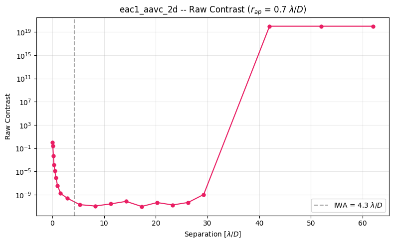
Contrast range: [9.24e-12, 1.00e+20]

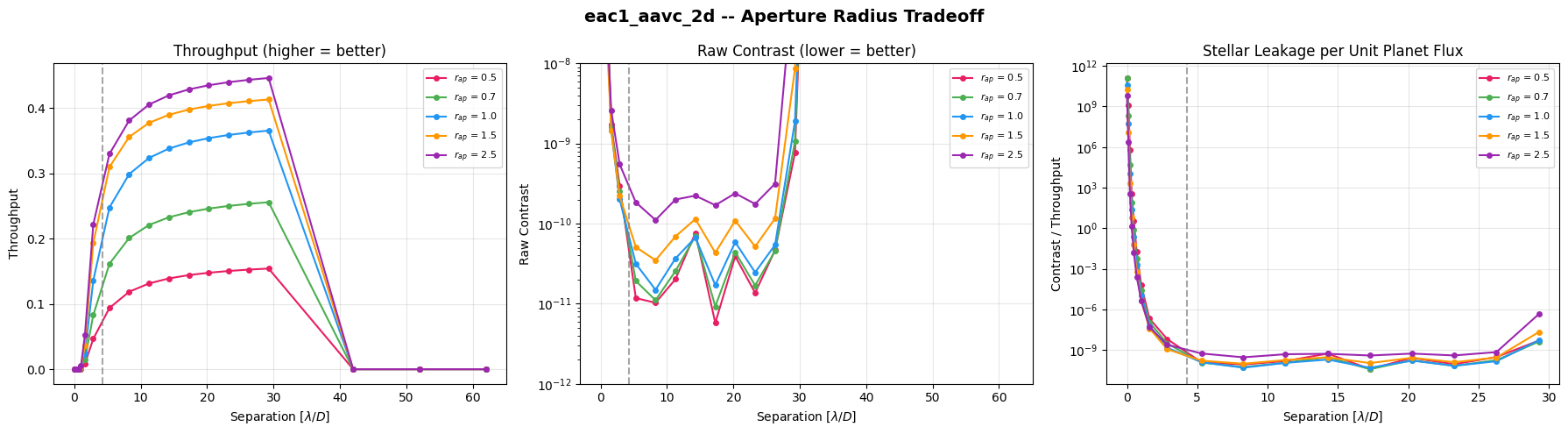
Contrast vs Aperture Radius

Show code cell source

Hide code cell source

radii = [0.5, 0.7, 1.0, 1.5, 2.5]
colors = ['#E91E63', '#4CAF50', '#2196F3', '#FF9800', '#9C27B0']

fig, axes = plt.subplots(1, 3, figsize=(18, 5))
ax_tp, ax_con, ax_ratio = axes

ref_sep, ref_tp = compute_throughput_curve(coro, aperture_radius_lod=0.7)
ref_sep_c, ref_con = compute_raw_contrast_curve(coro, aperture_radius_lod=0.7)

for r, c in zip(radii, colors, strict=True):
    s, t = compute_throughput_curve(coro, aperture_radius_lod=r)
    ax_tp.plot(s, t, 'o-', ms=4, color=c, label=f'$r_{{ap}}$ = {r}')

    s, con = compute_raw_contrast_curve(coro, aperture_radius_lod=r)
    ax_con.semilogy(s, con, 'o-', ms=4, color=c, label=f'$r_{{ap}}$ = {r}')

    # Contrast / throughput ratio (higher = worse)
    ax_ratio.semilogy(s, con / t, 'o-', ms=4, color=c, label=f'$r_{{ap}}$ = {r}')

for ax in axes:
    ax.axvline(coro.IWA.value, ls='--', color='gray', alpha=0.7)
    ax.legend(fontsize=8)
    ax.grid(True, alpha=0.3)
    ax.set_xlabel('Separation [$\\lambda/D$]')

ax_tp.set_ylabel('Throughput')
ax_tp.set_title('Throughput (higher = better)')

ax_con.set_ylabel('Raw Contrast')
ax_con.set_title('Raw Contrast (lower = better)')
# Zoom in to the relevant range
ax_con.set_ylim(1e-12, 1e-8)

ax_ratio.set_ylabel('Contrast / Throughput')
ax_ratio.set_title('Stellar Leakage per Unit Planet Flux')

fig.suptitle(f'{coro.name} -- Aperture Radius Tradeoff',
             fontsize=14, fontweight='bold')
plt.tight_layout()
plt.show()

/tmp/ipykernel_735/2337853976.py:18: RuntimeWarning: divide by zero encountered in divide
  ax_ratio.semilogy(s, con / t, 'o-', ms=4, color=c, label=f'$r_{{ap}}$ = {r}')

---

Core Mean Intensity

Core mean intensity \(\bar{I}_\star(r)\) is the azimuthally averaged stellar intensity at separation \(r\). It is computed by taking the radial profile of the on-axis (stellar) PSF – averaging the intensity in concentric annuli centered on the star.

This metric is used by EXOSIMS (primary method) and AYO/pyEDITH for computing the stellar leakage count rate. Unlike raw contrast, it does not depend on an aperture choice.

Radial Profile Animation

The animation below shows how the radial profile is measured: an annulus sweeps outward through the stellar PSF, and the mean intensity in each annulus builds up the \(\bar{I}_\star(r)\) curve.

Show code cell source

Hide code cell source

star_psf_0 = coro.stellar_intens(0.0 * lod)
center_y = coro.stellar_intens.center_y
center_x = coro.stellar_intens.center_x
pix_scale = coro.pixel_scale_arcsec.value

# Compute full radial profile
from hwoutils.radial import radial_profile
import jax.numpy as jnp

seps, profile = radial_profile(
    jnp.asarray(np.asarray(star_psf_0, dtype=np.float64)),
    pixel_scale_arcsec=pix_scale,
    center=(center_y, center_x),
    nbins=int(np.floor(np.max(star_psf_0.shape) / 2)),
)
seps = np.asarray(seps)
profile = np.asarray(profile)

# Only show up to OWA
owa_val = coro.OWA.value
mask_owa = seps <= owa_val * 1.1

# Build animation frames at each radial bin
# Sample every few bins to keep animation fast
step = max(1, len(seps[mask_owa]) // 25)
frame_indices = list(range(0, len(seps[mask_owa]), step))

fig_cmi = plt.figure(figsize=(14, 5))
gs_cmi = fig_cmi.add_gridspec(1, 2, width_ratios=[1, 1.3], wspace=0.3)
ax_psf = fig_cmi.add_subplot(gs_cmi[0, 0])
ax_prof = fig_cmi.add_subplot(gs_cmi[0, 1])

# Stellar PSF image
log_star = np.log10(np.maximum(star_psf_0, 1e-20))
vmax_s = log_star.max()
im_star = ax_psf.imshow(log_star, origin='lower', cmap='magma',
                        vmin=vmax_s - 8, vmax=vmax_s)
ax_psf.set_aspect('equal')

# Draw annulus
annulus_inner = plt.Circle((center_x, center_y), 0, fill=False,
                           ec='cyan', lw=2)
annulus_outer = plt.Circle((center_x, center_y), 0, fill=False,
                           ec='cyan', lw=2)
ax_psf.add_patch(annulus_inner)
ax_psf.add_patch(annulus_outer)
ax_psf.set_title('On-axis (stellar) PSF')
ax_psf.set_xlabel('x [pix]')
ax_psf.set_ylabel('y [pix]')

# Profile plot
ax_prof.semilogy(seps[mask_owa], profile[mask_owa], '-',
                 color='#CCCCCC', alpha=0.3, lw=2, zorder=1)
line_prof, = ax_prof.semilogy([], [], '-', color='#E91E63', lw=2, zorder=2)
dot_prof = ax_prof.scatter([], [], s=80, color='#E91E63', zorder=3)
ax_prof.axvline(coro.IWA.value, ls='--', color='gray', alpha=0.7,
                label=f'IWA = {coro.IWA.value:.1f}')
ax_prof.axvline(owa_val, ls='--', color='gray', alpha=0.5,
                label=f'OWA = {owa_val:.0f}')
ax_prof.set_xlabel('Separation [$\\lambda/D$]')
ax_prof.set_ylabel('Core Mean Intensity')
ax_prof.set_title('$\\bar{I}_\\star(r)$ -- Radial Profile')
ax_prof.legend()
ax_prof.grid(True, alpha=0.3)
ax_prof.set_xlim(0, owa_val * 1.1)

title_cmi = fig_cmi.suptitle('', fontsize=12)

def update_cmi(frame_num):
    idx = frame_indices[frame_num]
    r_lod = seps[idx]
    r_pix = r_lod / pix_scale
    dr_pix = (seps[1] - seps[0]) / pix_scale if idx > 0 else 1

    annulus_inner.set_radius(max(0, r_pix - dr_pix))
    annulus_outer.set_radius(r_pix + dr_pix)

    line_prof.set_data(seps[:idx+1], profile[:idx+1])
    dot_prof.set_offsets([[r_lod, profile[idx]]])

    title_cmi.set_text(
        f'Sep = {r_lod:.1f} $\\lambda/D$  |  '
        f'$\\bar{{I}}_\\star$ = {profile[idx]:.2e}'
    )
    return annulus_inner, annulus_outer, line_prof, dot_prof, title_cmi

anim_cmi = animation.FuncAnimation(fig_cmi, update_cmi,
                                   frames=len(frame_indices),
                                   interval=200, blit=False)
plt.close(fig_cmi)
HTML(anim_cmi.to_jshtml())

Once Loop Reflect

Effect of Stellar Diameter

The core mean intensity depends on the angular diameter of the host star. Larger stars produce broader stellar PSFs, which can leak more light into the dark hole. The animation below cycles through the available stellar diameters, showing how both the stellar PSF and the radial profile change.

Show code cell source

Hide code cell source

from hwoutils.radial import radial_profile
import jax.numpy as jnp

available_diams = coro.stellar_intens.diams
center_y = coro.stellar_intens.center_y
center_x = coro.stellar_intens.center_x
pix_scale = coro.pixel_scale_arcsec.value
owa_val = coro.OWA.value

# Pre-compute all PSFs and profiles
all_frames = []
for diam in available_diams:
    psf = coro.stellar_intens(diam)
    nbins = int(np.floor(np.max(psf.shape) / 2))
    s, p = radial_profile(
        jnp.asarray(np.asarray(psf, dtype=np.float64)),
        pixel_scale_arcsec=pix_scale,
        center=(center_y, center_x),
        nbins=nbins,
    )
    all_frames.append({
        'diam': diam,
        'psf': psf,
        'seps': np.asarray(s),
        'profile': np.asarray(p),
    })

# Keep only diameters with meaningfully different profiles.
# Compare each to the point-source baseline (not sequential neighbor).
baseline = all_frames[0]['profile']
diam_frames = [all_frames[0]]
for f in all_frames[1:]:
    max_rel_diff = np.max(np.abs(f['profile'] - baseline) / (np.abs(baseline) + 1e-30))
    if max_rel_diff > 0.01:
        diam_frames.append(f)

fig_diam = plt.figure(figsize=(14, 5))
gs_diam = fig_diam.add_gridspec(1, 2, width_ratios=[1, 1.3], wspace=0.3)
ax_psf_d = fig_diam.add_subplot(gs_diam[0, 0])
ax_prof_d = fig_diam.add_subplot(gs_diam[0, 1])

# Global colorscale for stellar PSF
global_star_peak = max(
    np.log10(np.maximum(f['psf'], 1e-20)).max() for f in diam_frames
)

f0 = diam_frames[0]
log_psf_d = np.log10(np.maximum(f0['psf'], 1e-20))
im_psf_d = ax_psf_d.imshow(log_psf_d, origin='lower', cmap='magma',
                            vmin=global_star_peak - 8, vmax=global_star_peak)
ax_psf_d.set_aspect('equal')
ax_psf_d.set_title('Stellar PSF')
ax_psf_d.set_xlabel('x [pix]')
ax_psf_d.set_ylabel('y [pix]')

# Plot all reference profiles in gray
for f in diam_frames:
    mask = f['seps'] <= owa_val
    ax_prof_d.semilogy(f['seps'][mask], f['profile'][mask], '-',
                       color='#CCCCCC', alpha=0.3, lw=1)

# Active profile line
mask0 = f0['seps'] <= owa_val
line_prof_d, = ax_prof_d.semilogy(f0['seps'][mask0], f0['profile'][mask0],
                                   '-', color='#E91E63', lw=2.5)
ax_prof_d.axvline(coro.IWA.value, ls='--', color='gray', alpha=0.7,
                  label=f'IWA = {coro.IWA.value:.1f}')
ax_prof_d.axvline(owa_val, ls='--', color='gray', alpha=0.5,
                  label=f'OWA = {owa_val:.0f}')
ax_prof_d.set_xlabel('Separation [$\\lambda/D$]')
ax_prof_d.set_ylabel('Core Mean Intensity')
ax_prof_d.set_title('Radial Profile')
ax_prof_d.legend()
ax_prof_d.grid(True, alpha=0.3)
ax_prof_d.set_xlim(0, owa_val)

title_diam = fig_diam.suptitle('', fontsize=13)

def update_diam(i):
    f = diam_frames[i]
    log_d = np.log10(np.maximum(f['psf'], 1e-20))
    im_psf_d.set_data(log_d)

    mask = f['seps'] <= owa_val
    line_prof_d.set_data(f['seps'][mask], f['profile'][mask])

    dval = f['diam'].value
    if dval < 0.01:
        label = 'Point source'
    else:
        label = f"$d_\\star$ = {dval:.2f} $\\lambda/D$"
    title_diam.set_text(f'Stellar Diameter: {label}')
    return im_psf_d, line_prof_d, title_diam

anim_diam = animation.FuncAnimation(fig_diam, update_diam,
                                    frames=len(diam_frames),
                                    interval=800, blit=False)
plt.close(fig_diam)
HTML(anim_diam.to_jshtml())

Once Loop Reflect