Core Throughput

Core throughput measures how much of the planet’s light survives the coronagraph and lands in the photometric aperture. It directly scales the planet count rate in the ETC.

Theory

Coronagraphic PSF

The coronagraphic PSF \(\text{PSF}_{\text{coro}}(x, x_0, \lambda)\) is the system response with all coronagraph masks in place and the system optimized to suppress starlight in the dark hole. Unlike a conventional PSF, it varies with the off-axis source position \(x_0\).

Absolute Throughput

Coronagraph throughput \(\eta_p\) is the fraction of available planet light detected. It is computed by integrating \(\text{PSF}_{\text{coro}}\) centered on \(x_0\) over the photometric aperture \(\text{AP}(x_0)\):

\[\Upsilon_c(r) = \frac{\text{flux in aperture at separation } r}{\text{total PSF flux}}\]

In the ETC, throughput directly scales the planet count rate \(C_p\).

API: Use compute_throughput_curve() to get throughput as a function of separation, or the stored interpolator via coro.throughput(separation).

from yippy.performance import compute_throughput_curve
seps, throughputs = compute_throughput_curve(coro, aperture_radius_lod=0.7)
# Or use the interpolator directly:
tp = coro.throughput(8.0)  # throughput at 8 lam/D

Show code cell source

Hide code cell source

import matplotlib.pyplot as plt
import numpy as np
from matplotlib.patches import Circle
from matplotlib import animation
from IPython.display import HTML
from yippy import fetch_yip
from yippy import Coronagraph
from yippy.performance import (
    compute_throughput_curve,
    compute_truncation_throughput_curve,
    compute_truncation_core_area_curve,
    _iter_xaxis_positions,
    _point_source_in_image,
    _threshold_mask,
    _oversample_psf,
)
from yippy.util import extract_and_oversample_subarray, measure_flux_in_oversampled_aperture

import logging; logging.getLogger("yippy").setLevel(logging.ERROR)

yip_path = fetch_yip("eac1_aavc_2d")
coro = Coronagraph(yip_path)
print(f"Coronagraph: {coro.name} (Amplitude Apodized Vortex Coronagraph, generated by Susan Redmond)")
print(f"Pixel scale: {coro.pixel_scale_arcsec}")
print(f"IWA: {coro.IWA:.2f}, OWA: {coro.OWA:.2f}")

/home/docs/checkouts/readthedocs.org/user_builds/yippy/envs/latest/lib/python3.12/site-packages/tqdm/auto.py:21: TqdmWarning: IProgress not found. Please update jupyter and ipywidgets. See https://ipywidgets.readthedocs.io/en/stable/user_install.html
  from .autonotebook import tqdm as notebook_tqdm

Coronagraph: eac1_aavc_2d (Amplitude Apodized Vortex Coronagraph, generated by Susan Redmond)
Pixel scale: 0.25 λ/D / pix
IWA: 4.26 λ/D, OWA: 32.00 λ/D

---

Fixed Circular Aperture

The default approach uses a fixed circular aperture (typically 0.7 \(\lambda/D\)) centered on the PSF peak at each off-axis position. This is the standard method used by EXOSIMS.

Calculation Walkthrough

The compute_throughput_curve function:

1. Iterates over each off-axis PSF position along the x-axis

2. Extracts and oversamples a subarray around the PSF peak

3. Places a circular aperture centered on the PSF peak

4. Sums the flux inside the aperture (PSF is normalized to 1)

The animation below shows this process at each PSF position, building up the throughput curve point by point.

Show code cell source

Hide code cell source

aperture_radius_lod = 0.7
oversample = 2
radius_pix = aperture_radius_lod / coro.pixel_scale_arcsec.value

positions = [p for p in _iter_xaxis_positions(coro) if _point_source_in_image(p)]

frames = []
for pos in positions:
    sub_os, px_os, py_os, r_os, sub_orig = extract_and_oversample_subarray(
        pos.psf, pos.px, pos.py, radius_pix, oversample
    )
    flux = measure_flux_in_oversampled_aperture(sub_os, px_os, py_os, r_os, sub_orig)
    frames.append({
        'sep': pos.separation,
        'full_psf': pos.psf,
        'px': pos.px, 'py': pos.py,
        'sub_os': sub_os,
        'cx': px_os, 'cy': py_os,
        'r_os': r_os,
        'throughput': flux,
    })

# Compute global colorscale across all frames
global_peak_full = max(
    np.log10(np.maximum(f['full_psf'], 1e-20)).max() for f in frames
)
global_peak_zoom = max(
    np.log10(np.maximum(f['sub_os'], 1e-20)).max() for f in frames
)

fig = plt.figure(figsize=(18, 5))
gs = fig.add_gridspec(1, 3, width_ratios=[1, 1, 1.2], wspace=0.3)
ax_full = fig.add_subplot(gs[0, 0])
ax_zoom = fig.add_subplot(gs[0, 1])
ax_curve = fig.add_subplot(gs[0, 2])

# Full-frame PSF
f0 = frames[0]
log_full = np.log10(np.maximum(f0['full_psf'], 1e-20))

im_full = ax_full.imshow(log_full, origin='lower', cmap='magma',
                         vmin=global_peak_full - 5, vmax=global_peak_full)
circ_full = plt.Circle((f0['px'], f0['py']), radius_pix,
                       fill=False, ec='cyan', lw=2, ls='--')
ax_full.add_patch(circ_full)
ax_full.set_title('Off-axis PSF (full frame)')
ax_full.set_aspect('equal')
ax_full.set_xlabel('x [pix]')
ax_full.set_ylabel('y [pix]')

# Zoomed subarray
log_zoom = np.log10(np.maximum(f0['sub_os'], 1e-20))
vmax_zoom = log_zoom.max()
im_zoom = ax_zoom.imshow(log_zoom, origin='lower', cmap='magma',
                         vmin=global_peak_zoom - 4, vmax=global_peak_zoom)
circ_zoom = plt.Circle((f0['cx'], f0['cy']), f0['r_os'],
                       fill=False, ec='cyan', lw=2, ls='--')
ax_zoom.add_patch(circ_zoom)
ax_zoom.set_title('Zoomed (2x oversampled)')
ax_zoom.set_aspect('equal')
ax_zoom.set_xlabel('x [oversampled pix]')

title_fig = fig.suptitle('', fontsize=12)

# Throughput curve
seps_all = [f['sep'] for f in frames]
tp_all = [f['throughput'] for f in frames]
ax_curve.plot(seps_all, tp_all, 'o-', ms=4, color='#CCCCCC', alpha=0.3, zorder=1)
scatter = ax_curve.scatter([], [], s=80, color='#4CAF50', zorder=3)
line_built, = ax_curve.plot([], [], 'o-', ms=5, color='#4CAF50', zorder=2)
ax_curve.axvline(coro.IWA.value, ls='--', color='gray', alpha=0.7,
                 label=f'IWA = {coro.IWA.value:.1f}')
ax_curve.set_xlabel('Separation [$\\lambda/D$]')
ax_curve.set_ylabel('Throughput')
ax_curve.set_title('Throughput Curve')
ax_curve.legend()
ax_curve.grid(True, alpha=0.3)

def update(i):
    f = frames[i]
    # Update full-frame
    log_f = np.log10(np.maximum(f['full_psf'], 1e-20))
    im_full.set_data(log_f)
    circ_full.set_center((f['px'], f['py']))

    # Update zoom
    log_z = np.log10(np.maximum(f['sub_os'], 1e-20))
    im_zoom.set_data(log_z)
    im_zoom.set_extent([-0.5, log_z.shape[1]-0.5, -0.5, log_z.shape[0]-0.5])
    ax_zoom.set_xlim(-0.5, log_z.shape[1]-0.5)
    ax_zoom.set_ylim(-0.5, log_z.shape[0]-0.5)
    circ_zoom.set_center((f['cx'], f['cy']))
    circ_zoom.set_radius(f['r_os'])

    title_fig.set_text(
        f"Sep = {f['sep']:.2f} $\\lambda/D$  |  "
        f"Throughput = {f['throughput']:.4f}"
    )

    line_built.set_data(seps_all[:i+1], tp_all[:i+1])
    scatter.set_offsets([[f['sep'], f['throughput']]])
    return im_full, im_zoom, circ_full, circ_zoom, title_fig, line_built, scatter

anim = animation.FuncAnimation(fig, update, frames=len(frames), interval=400, blit=False)
plt.close(fig)
HTML(anim.to_jshtml())

Once Loop Reflect

Throughput Curve

Show code cell source

Hide code cell source

sep, throughput = compute_throughput_curve(coro, aperture_radius_lod=0.7)

fig, ax = plt.subplots(figsize=(8, 5))
ax.plot(sep, throughput, 'o-', ms=5, color='#4CAF50')
ax.axvline(coro.IWA.value, ls='--', color='gray', alpha=0.7,
           label=f'IWA = {coro.IWA.value:.1f} $\\lambda/D$')
ax.set_xlabel('Separation [$\\lambda/D$]')
ax.set_ylabel('Throughput')
ax.set_title(f'{coro.name} -- Core Throughput ($r_{{ap}}$ = 0.7 $\\lambda/D$)')
ax.legend()
ax.grid(True, alpha=0.3)
plt.tight_layout()
plt.show()

print(f"Number of PSF positions: {len(sep)}")
print(f"Throughput range: [{throughput.min():.4f}, {throughput.max():.4f}]")

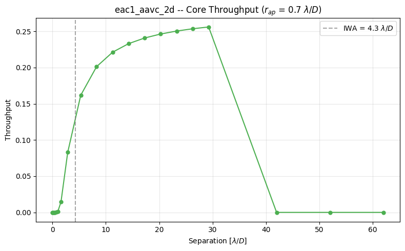
Number of PSF positions: 21
Throughput range: [0.0000, 0.2560]

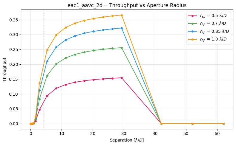
Aperture Radius Effect

The choice of aperture radius affects throughput directly. Larger apertures capture more planet flux (higher throughput) but also more background and stellar leakage. This tradeoff is explored in the contrast notebook.

Show code cell source

Hide code cell source

radii = [0.5, 0.7, 0.85, 1.0]
colors = ['#E91E63', '#4CAF50', '#2196F3', '#FF9800']

fig, ax = plt.subplots(figsize=(8, 5))

for r, c in zip(radii, colors, strict=True):
    s, t = compute_throughput_curve(coro, aperture_radius_lod=r)
    ax.plot(s, t, 'o-', ms=4, color=c, label=f'$r_{{ap}}$ = {r} $\\lambda/D$')

ax.axvline(coro.IWA.value, ls='--', color='gray', alpha=0.7)
ax.set_xlabel('Separation [$\\lambda/D$]')
ax.set_ylabel('Throughput')
ax.set_title(f'{coro.name} -- Throughput vs Aperture Radius')
ax.legend()
ax.grid(True, alpha=0.3)
plt.tight_layout()
plt.show()

---

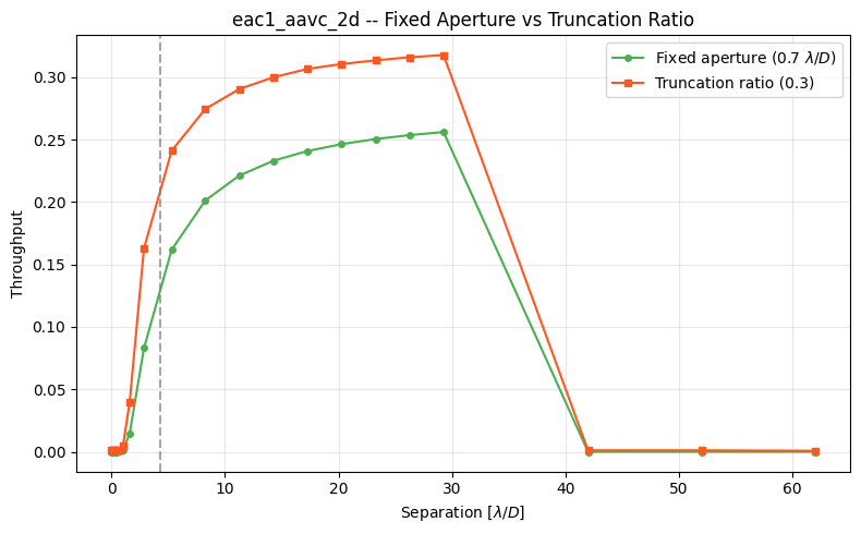
PSF Truncation Ratio (AYO Mode)

AYO uses a fundamentally different aperture strategy: instead of a fixed circular aperture, it selects all pixels where the PSF exceeds a fraction of its peak value. This adaptive aperture changes shape and size with separation.

\[\begin{split}\text{mask}(x, y) = \begin{cases} 1 & \text{if PSF}(x,y) > \text{ratio} \times \text{peak} \\ 0 & \text{otherwise} \end{cases}\end{split}\]

AYO’s ETC loops over multiple truncation ratios and picks the one that minimizes integration time at each separation.

Truncation Mask Animation

The animation below shows the truncation mask (red contour) sweeping through PSF positions. Unlike the fixed circular aperture, the mask shape adapts to the PSF structure at each separation.

Show code cell source

Hide code cell source

psf_trunc_ratio = 0.3
pix_lod = coro.pixel_scale_arcsec.value
os_factor = int(np.ceil(pix_lod / 0.05))
crop_radius = int(5 / (pix_lod / os_factor))  # +/-5 lam/D

from yippy.util import crop_around_peak

trunc_frames = []
for pos in positions:
    psf_os_full = _oversample_psf(pos.psf, pix_lod, os_factor)
    mask_full = _threshold_mask(psf_os_full, psf_trunc_ratio)
    tp = psf_os_full[mask_full].sum()
    # Crop both arrays centered on the PSF peak
    psf_os = crop_around_peak(psf_os_full, crop_radius)
    # Crop mask with the same window
    peak_y, peak_x = np.unravel_index(psf_os_full.argmax(), psf_os_full.shape)
    ny, nx = psf_os_full.shape
    r = min(crop_radius, peak_y, ny - peak_y, peak_x, nx - peak_x)
    mask = mask_full[peak_y - r:peak_y + r, peak_x - r:peak_x + r]
    trunc_frames.append({
        'sep': pos.separation,
        'full_psf': pos.psf,
        'psf_os': psf_os,
        'mask': mask,
        'throughput': tp,
    })

# Compute global colorscale across all frames
global_peak_full2 = max(
    np.log10(np.maximum(f['full_psf'], 1e-20)).max() for f in trunc_frames
)
global_peak_mask = max(
    np.log10(np.maximum(f['psf_os'], 1e-20)).max() for f in trunc_frames
)

fig2 = plt.figure(figsize=(18, 5))
gs2 = fig2.add_gridspec(1, 3, width_ratios=[1, 1, 1.2], wspace=0.3)
ax_full2 = fig2.add_subplot(gs2[0, 0])
ax_mask = fig2.add_subplot(gs2[0, 1])
ax_tc = fig2.add_subplot(gs2[0, 2])

# Full-frame PSF
f0 = trunc_frames[0]
log_full2 = np.log10(np.maximum(f0['full_psf'], 1e-20))
im_full2 = ax_full2.imshow(log_full2, origin='lower', cmap='magma',
                           vmin=global_peak_full2 - 5, vmax=global_peak_full2)
ax_full2.set_title('Off-axis PSF (full frame)')
ax_full2.set_xlabel('x [pix]')
ax_full2.set_ylabel('y [pix]')
ax_full2.set_aspect('equal')

# Cropped oversampled PSF with truncation mask
log_psf = np.log10(np.maximum(f0['psf_os'], 1e-20))
im_mask = ax_mask.imshow(log_psf, origin='lower', cmap='magma',
                         vmin=global_peak_mask - 4, vmax=global_peak_mask)
contour_set = ax_mask.contour(f0['mask'].astype(float), levels=[0.5],
                             colors='cyan', linewidths=2)
ax_mask.set_title('Truncation mask (zoomed)')
ax_mask.set_xlabel('x [oversampled pix]')
ax_mask.set_aspect('equal')

title_mask = fig2.suptitle('', fontsize=12)

# Throughput curve
t_seps = [f['sep'] for f in trunc_frames]
t_tps = [f['throughput'] for f in trunc_frames]
ax_tc.plot(t_seps, t_tps, 'o-', ms=4, color='#CCCCCC', alpha=0.3, zorder=1)
scatter2 = ax_tc.scatter([], [], s=80, color='#FF5722', zorder=3)
line_built2, = ax_tc.plot([], [], 'o-', ms=5, color='#FF5722', zorder=2)
ax_tc.axvline(coro.IWA.value, ls='--', color='gray', alpha=0.7,
              label=f'IWA = {coro.IWA.value:.1f}')
ax_tc.set_xlabel('Separation [$\\lambda/D$]')
ax_tc.set_ylabel('Throughput')
ax_tc.set_title(f'Truncation Throughput (ratio = {psf_trunc_ratio})')
ax_tc.legend()
ax_tc.grid(True, alpha=0.3)

def update_trunc(i):
    f = trunc_frames[i]

    # Update full-frame
    log_f = np.log10(np.maximum(f['full_psf'], 1e-20))
    im_full2.set_data(log_f)

    # Update cropped mask view
    log_img = np.log10(np.maximum(f['psf_os'], 1e-20))
    im_mask.set_data(log_img)
    im_mask.set_extent([-0.5, log_img.shape[1]-0.5, -0.5, log_img.shape[0]-0.5])
    ax_mask.set_xlim(-0.5, log_img.shape[1]-0.5)
    ax_mask.set_ylim(-0.5, log_img.shape[0]-0.5)

    for coll in ax_mask.collections[:]:
        coll.remove()
    ax_mask.contour(f['mask'].astype(float), levels=[0.5],
                   colors='cyan', linewidths=2)

    n_pix = f['mask'].sum()
    title_mask.set_text(
        f"Sep = {f['sep']:.2f} $\\lambda/D$  |  "
        f"Mask pixels: {n_pix}  |  Throughput: {f['throughput']:.4f}"
    )

    line_built2.set_data(t_seps[:i+1], t_tps[:i+1])
    scatter2.set_offsets([[f['sep'], f['throughput']]])
    return im_full2, im_mask, title_mask, line_built2, scatter2

anim2 = animation.FuncAnimation(fig2, update_trunc, frames=len(trunc_frames),
                                interval=400, blit=False)
plt.close(fig2)
HTML(anim2.to_jshtml())

Once Loop Reflect

Fixed Aperture vs Truncation Ratio Comparison

Show code cell source

Hide code cell source

sep_f, tp_fixed = compute_throughput_curve(coro, aperture_radius_lod=0.7)
sep_tr, tp_trunc = compute_truncation_throughput_curve(coro, psf_trunc_ratio=0.3)

fig, ax = plt.subplots(figsize=(8, 5))
ax.plot(sep_f, tp_fixed, 'o-', ms=4, color='#4CAF50',
        label='Fixed aperture (0.7 $\\lambda/D$)')
ax.plot(sep_tr, tp_trunc, 's-', ms=4, color='#FF5722',
        label='Truncation ratio (0.3)')
ax.axvline(coro.IWA.value, ls='--', color='gray', alpha=0.7)
ax.set_xlabel('Separation [$\\lambda/D$]')
ax.set_ylabel('Throughput')
ax.set_title(f'{coro.name} -- Fixed Aperture vs Truncation Ratio')
ax.legend()
ax.grid(True, alpha=0.3)
plt.tight_layout()
plt.show()