Noise Floors and Integration Time

This notebook ties all the metrics together, showing how they determine the final signal-to-noise ratio and exposure time. The key concept is the noise floor: a systematic limit below which no amount of integration time can improve detection.

Two Noise Floor Conventions

Both ETCs ultimately produce the same noise floor count rate, but they store the intermediate value differently:

• EXOSIMS stores the noise floor in contrast units: \(\text{NF}_{\text{EXOSIMS}} = C_{\text{raw}} / \text{ppf}\). The ETC multiplies by throughput to recover the count rate. This is EXOSIMS’s fallback path, used when core_mean_intensity is not provided.

• AYO stores the noise floor in per-pixel intensity units: \(\text{NF}_{\text{AYO}} = \bar{I}_\star / \text{ppf}\). The ETC multiplies by \(\Omega / \theta_{\text{pix}}^2\) to scale from per-pixel to per-aperture.

The algebraic relationship between them:

\[\text{NF}_{\text{EXOSIMS}} = \text{NF}_{\text{AYO}} \cdot \frac{\Omega}{\theta_{\text{pix}}^2 \cdot \eta_p}\]

For a detailed derivation, worked examples, and the distinction between EXOSIMS’s standard and fallback code paths, see Noise Floor Conventions.

Show code cell source

Hide code cell source

import matplotlib.pyplot as plt
import numpy as np
from yippy import fetch_yip
from yippy import Coronagraph

import logging; logging.getLogger("yippy").setLevel(logging.ERROR)

yip_path = fetch_yip("eac1_aavc_2d")
coro = Coronagraph(yip_path)
print(f"Coronagraph: {coro.name} (Amplitude Apodized Vortex Coronagraph, generated by Susan Redmond)")
print(f"IWA: {coro.IWA:.2f}, OWA: {coro.OWA:.2f}")

/home/docs/checkouts/readthedocs.org/user_builds/yippy/envs/stable/lib/python3.12/site-packages/tqdm/auto.py:21: TqdmWarning: IProgress not found. Please update jupyter and ipywidgets. See https://ipywidgets.readthedocs.io/en/stable/user_install.html
  from .autonotebook import tqdm as notebook_tqdm

Coronagraph: eac1_aavc_2d (Amplitude Apodized Vortex Coronagraph, generated by Susan Redmond)
IWA: 4.26 λ/D, OWA: 32.00 λ/D

---

Noise Floor Comparison

yippy provides two noise floor conventions, matching the two ETC families:

• EXOSIMS: coro.noise_floor_exosims(r) – bounds noise in contrast units (per-aperture, divided by throughput)

• AYO / pyEDITH: coro.noise_floor_ayo(r) – bounds noise in per-pixel intensity units

For the full mathematical derivation of both conventions, see Noise Floor Conventions.

Show code cell source

Hide code cell source

seps = np.linspace(coro.IWA.value, coro.OWA.value, 200)

# Default (clamped) and unclamped noise floors
nf_exosims_clamped = coro.noise_floor_exosims(seps)
nf_exosims_true = coro.noise_floor_exosims(seps, contrast_floor=0)
nf_ayo = coro.noise_floor_ayo(seps)

fig, (ax1, ax2) = plt.subplots(1, 2, figsize=(14, 5))

ax1.semilogy(seps, nf_exosims_clamped, color='#E91E63', lw=2,
             label='Clamped (default)')
ax1.semilogy(seps, nf_exosims_true, color='#E91E63', lw=1.5,
             ls='--', alpha=0.6, label='Unclamped')
ax1.axhline(1e-10 / 30, color='gray', ls=':', lw=1, alpha=0.5,
            label=f'$C_{{floor}}$ / ppf = {1e-10/30:.1e}')
ax1.set_xlabel('Separation [$\\lambda/D$]')
ax1.set_ylabel('NF (contrast units)')
ax1.set_title('EXOSIMS Convention')
ax1.legend(fontsize=8)
ax1.grid(True, alpha=0.3)

ax2.semilogy(seps, nf_ayo, color='#FF9800', lw=2)
ax2.set_xlabel('Separation [$\\lambda/D$]')
ax2.set_ylabel('NF (intensity units)')
ax2.set_title('AYO Convention')
ax2.grid(True, alpha=0.3)

fig.suptitle(f'{coro.name} -- Noise Floor Conventions (ppf = 30)',
             fontsize=14, fontweight='bold')
plt.tight_layout()
plt.show()

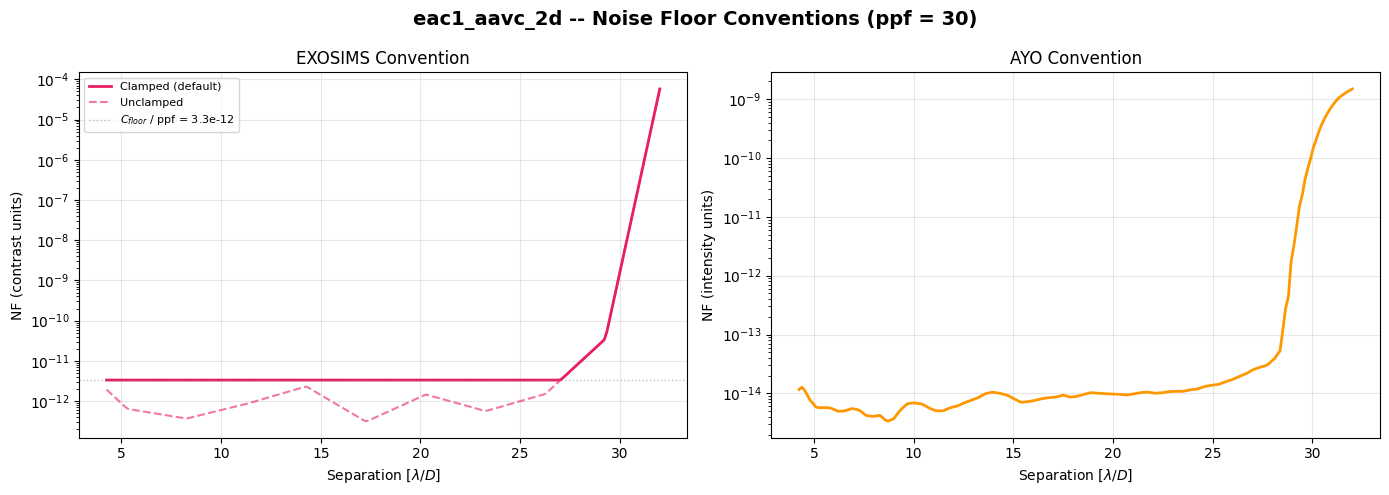
The EXOSIMS curve (left, dashed) is noticeably noisier than the AYO curve (right). This is because raw contrast divides CMI by throughput: \(C_{\text{raw}} = \bar{I}_\star \Omega / (\theta_{\text{pix}}^2 \eta_p)\). Throughput is computed from aperture photometry on the discrete off-axis PSFs provided in the YIP, then interpolated. This sparse sampling introduces the jagged oscillations that are amplified when dividing. The AYO convention avoids this since it stores \(\bar{I}_\star\) directly – a smooth radial average of the full 2D stellar intensity map.

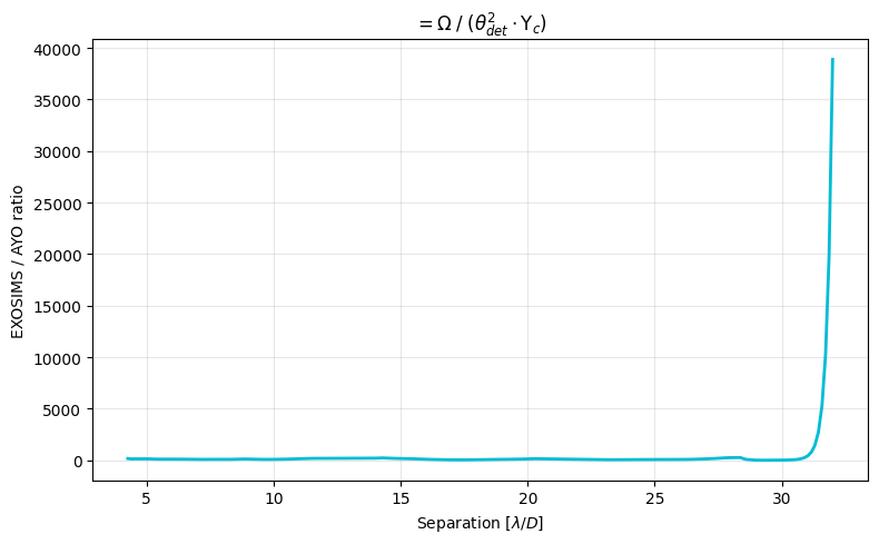
Convention Ratio

The ratio between the two conventions reveals the geometric factor \(\Omega / (\theta_{det}^2 \cdot \Upsilon_c)\):

Show code cell source

Hide code cell source

ratio = nf_exosims_true / nf_ayo

fig, ax = plt.subplots(figsize=(8, 5))
ax.plot(seps, ratio, color='#00BCD4', lw=2)
ax.set_xlabel('Separation [$\\lambda/D$]')
ax.set_ylabel('EXOSIMS / AYO ratio')
ax.set_title('$= \\Omega \\; / \\; (\\theta_{det}^2 \\cdot \\Upsilon_c)$')
ax.grid(True, alpha=0.3)
plt.tight_layout()
plt.show()

---

Integration Time Equations

The noise floor enters the integration time equation in the denominator. When the planet signal approaches the noise floor, the denominator approaches zero and \(t_{\text{int}} \to \infty\).

EXOSIMS

\[t_{\text{int}} = \frac{\bar{c}_p + \bar{c}_b}{\left(\frac{\bar{c}_p}{\text{SNR}}\right)^2 - \bar{c}_{sp}^2}\]

where \(\bar{c}_{sp} = \bar{c}_{sr} \cdot \text{ppFact} \cdot \text{stabilityFact}\). This is the default OpticalSystem formulation. The Nemati module additionally scales \(\bar{c}_b\) by RDI reference star factors \(k_{SZ}\) and \(k_{det}\).

AYO / pyEDITH

\[t_{\text{int}} = \frac{C_p + 2\, C_b}{\left(\frac{C_p}{\text{SNR}}\right)^2 - C_{nf}^2}\]

where the factor of 2 accounts for ADI background subtraction.

Integration Time Divergence

Show code cell source

Hide code cell source

seps = np.linspace(coro.IWA.value, coro.OWA.value, 200)
snr_target = 7.0

tp = coro.throughput(seps)
nf = coro.noise_floor_ayo(seps)

planet_signals = np.logspace(-3, 0, 50)

fig, ax = plt.subplots(figsize=(8, 5))

sample_seps = [5.0, 10.0, 20.0]
colors = ['#E91E63', '#4CAF50', '#2196F3']

for sep_val, color in zip(sample_seps, colors, strict=True):
    nf_val = float(coro.noise_floor_ayo(sep_val))
    tp_val = float(coro.throughput(sep_val))

    c_p = planet_signals * tp_val
    c_nf = nf_val

    denom = (c_p / snr_target) ** 2 - c_nf ** 2
    valid = denom > 0
    t_int = np.full_like(c_p, np.inf)
    t_int[valid] = c_p[valid] / denom[valid]

    ax.semilogy(planet_signals[valid], t_int[valid], '-', color=color, lw=2,
               label=f'r = {sep_val:.0f} $\\lambda/D$')

    diverge_signal = snr_target * c_nf / tp_val
    if diverge_signal < planet_signals.max():
        ax.axvline(diverge_signal, ls=':', color=color, alpha=0.5)

ax.set_xlabel('Relative Planet Signal')
ax.set_ylabel('Integration Time (arb. units)')
ax.set_title(f'{coro.name} -- Integration Time vs Planet Signal\n'
             f'(SNR = {snr_target}, AYO convention)')
ax.legend()
ax.grid(True, alpha=0.3)
plt.tight_layout()
plt.show()

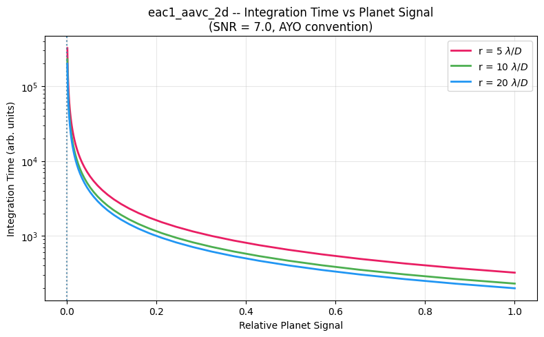
The vertical dotted lines mark where integration time diverges. Planets fainter than these thresholds are fundamentally undetectable at the given separation, regardless of observation duration.

---

See also:

• Noise Floor Conventions for the full algebraic derivation

• Performance Metrics Overview for the complete ETC variable mapping