Aperture Photometry: Fixed Circle vs PSF Truncation#

This notebook compares two approaches to defining the photometric aperture for coronagraphic performance metrics:

	EXOSIMS (Fixed Aperture)	AYO / pyEDITH (Truncation Mask)
Shape	Circular, radius \(r_{ap}\)	Adaptive, PSF > ratio \(\times\) peak
Throughput	Flux in circle / total flux	Flux above threshold / total flux
Stellar Noise	\(C(r) \cdot \Upsilon_c(r)\) (contrast \(\times\) core area)	\(\bar{I}_\star \cdot \Omega\) (intensity \(\times\) core area)
Core Area	\(\pi r_{ap}^2\) (fixed)	\(\sum_{\text{mask}} \Delta\theta^2\) (varies with separation)
Free Parameter	Aperture radius \(r_{ap}\)	Truncation ratio

The key question: how does the choice of photometric region affect the throughput-to-noise tradeoff?

/home/docs/checkouts/readthedocs.org/user_builds/yippy/envs/stable/lib/python3.12/site-packages/tqdm/auto.py:21: TqdmWarning: IProgress not found. Please update jupyter and ipywidgets. See https://ipywidgets.readthedocs.io/en/stable/user_install.html
  from .autonotebook import tqdm as notebook_tqdm

Coronagraph: eac1_aavc_2d
IWA: 4.26 λ/D, OWA: 32.00 λ/D
Pixel scale: 0.2500 λ/D / pix

API: The functions used in this notebook are from yippy.performance:

from yippy.performance import (
    compute_throughput_curve,          # fixed aperture throughput
    compute_raw_contrast_curve,        # fixed aperture raw contrast
    compute_truncation_throughput_curve,  # truncation throughput
    compute_truncation_core_area_curve,   # truncation core area
    compute_core_mean_intensity_curve,    # stellar intensity profile
)

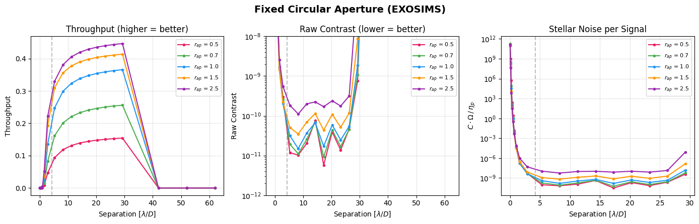
Fixed Circular Aperture (EXOSIMS)#

EXOSIMS uses a circular aperture of fixed radius \(r_{ap}\) (in \(\lambda/D\)) centered on the expected planet position. The same circle is used for both the planet PSF (throughput) and the stellar PSF (raw contrast).

The core area is simply \(\Omega = \pi r_{ap}^2\), independent of separation.

/tmp/ipykernel_869/85225529.py:12: RuntimeWarning: divide by zero encountered in divide
  noise_per_signal = con * omega / tp

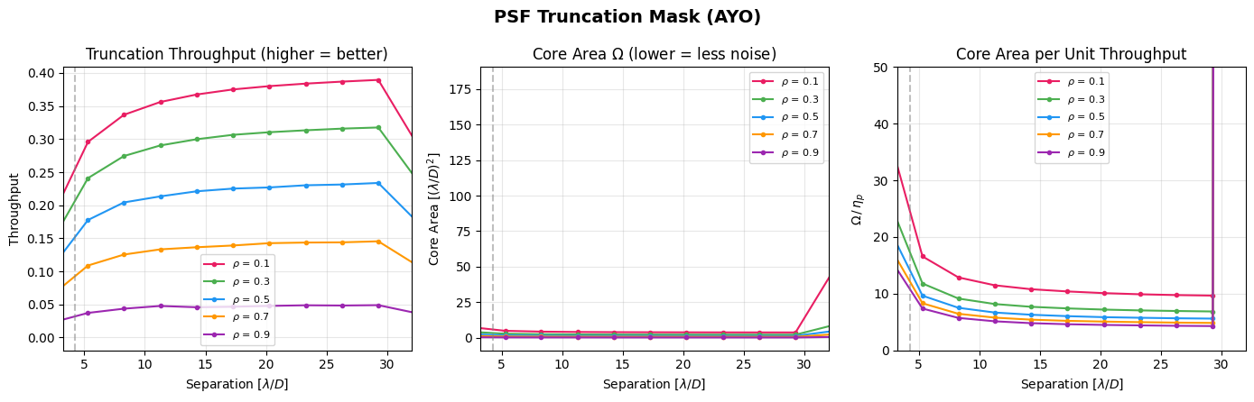
../_images/21b14c22cadbc725af8409d977342576ec357d77f6dd4ec1e7195888b65a56e4.png

PSF Truncation Mask (AYO)#

AYO defines the photometric region as all pixels where the off-axis PSF exceeds a fraction (the truncation ratio) of its peak value. This produces an adaptive aperture that follows the PSF shape:

\[\begin{split}\text{mask}(x,y) = \begin{cases} 1 & \text{if } \text{PSF}(x,y) > \rho \cdot \text{PSF}_{\max} \\ 0 & \text{otherwise} \end{cases}\end{split}\]

The core area \(\Omega = \sum_{\text{mask}} (\Delta\theta)^2\) varies with separation because the PSF shape changes across the focal plane.

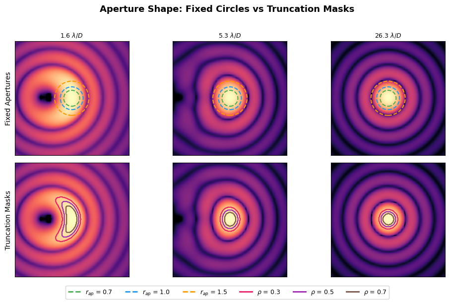
../_images/359c980aa674232eaf876db33809d332e6053fa87b4eb1666d268fa1cf7d9761.png

Side-by-Side: Aperture Shape Comparison#

Both methods define an aperture and measure throughput within it. The key difference: the truncation mask adapts to the PSF shape, while the fixed circle does not. Let’s visualize both at several separations.

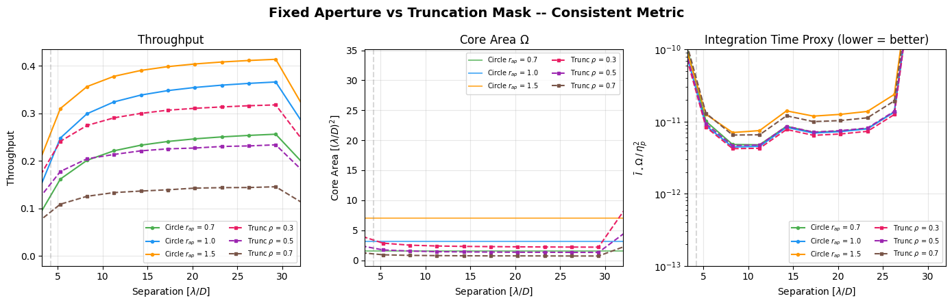
../_images/dfb5d5a3d3acbc79e7823d2f5fb837f3eb5496d32b8914d6900d23889a7be18d.png

Consistent Noise Metric#

To compare both methods on equal footing, we need the same noise proxy. The ETC integration time for stellar-noise-limited observations scales as:

\[t_{\text{int}} \propto \frac{\bar{I}_\star(r) \cdot \Omega}{\eta_p^2}\]

where \(\bar{I}_\star\) is the core mean intensity (same for both methods since it depends only on the stellar PSF, not the aperture choice), \(\Omega\) is the core area, and \(\eta_p\) is the throughput.

This metric is consistent because it uses:

For fixed apertures: \(\Omega = \pi r_{ap}^2\) and \(\eta_p\) from circular photometry
For truncation masks: \(\Omega = \sum_{\text{mask}} \Delta\theta^2\) and \(\eta_p\) from threshold photometry

The stellar intensity \(\bar{I}_\star\) is the same for both, so it cancels in relative comparisons.

/tmp/ipykernel_869/2734778706.py:17: RuntimeWarning: divide by zero encountered in divide
  noise = i_star_at_s * omega / tp**2

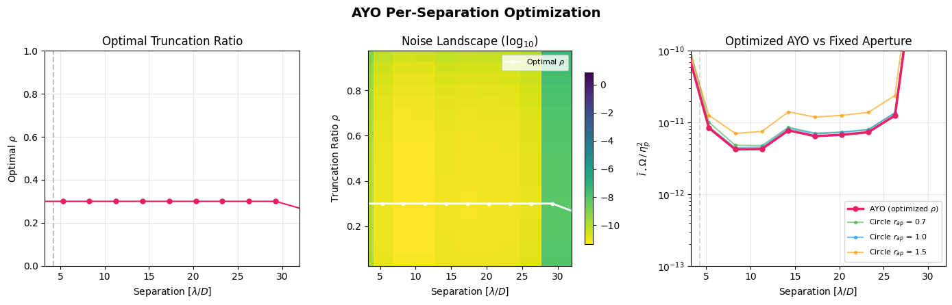
../_images/852ed61b61277b8c3e2ad607461231c9b08ce396935a63658ac27a105b71dc32.png

AYO’s Per-Separation Optimization#

The comparison above uses fixed truncation ratios, but AYO optimizes the truncation ratio at each planet position to minimize integration time. In calc_exp_time, AYO loops over all available truncation ratios for each planet and keeps the one that yields the shortest exposure time:

for (iratio = 0; iratio < npsfratios; iratio++) {
    CRp = tempCRpfactor * photap_frac[index2];      // signal
    CRb = tempCRbfactor * omega_lod[index2];         // all background noise
    CRbd = CRbdfactor * det_npix;                    // detector noise
    cp = (CRp + 2*CRb) / (CRp^2 - CRnf^2);         // exposure factor
    if (temptp < besttp_v_ratio)
        besttp_v_ratio = temptp;                     // keep the best
}

All noise terms – stellar leakage, zodiacal, exozodiacal, binary contamination, thermal, and detector noise – scale with omega_lod (core area). Signal scales with photap_frac (throughput).

Our simplified proxy \(\bar{I}_\star \Omega / \eta_p^2\) captures the dominant tradeoff. The figure below shows the optimization results:

/tmp/ipykernel_869/2722695700.py:71: RuntimeWarning: divide by zero encountered in divide
  noise_fix = i_star_s * omega / tp**2

../_images/ca64d1e17d2040ac709739e7f3fe056861518003bb7a8d4fc62eeaed7291eb0f.png

Discussion#

Key Finding: The Optimal Ratio is Separation-Independent#

The optimization sweep reveals that the optimal truncation ratio is constant across all separations for this coronagraph. This follows from the structure of AYO’s ETC:

All noise terms scale as \(\Omega(\rho)\)
Planet signal scales as \(\eta_p(\rho)\)
Position-dependent factors (\(\bar{I}_\star\), sky transmission, etc.) are independent of \(\rho\)

So the optimal \(\rho\) at each position depends only on \(\Omega(\rho) / \eta_p(\rho)^2\), which is a property of the PSF core shape. For this coronagraph, the PSF shape is stable across the working region, producing a uniform optimal \(\rho \approx 0.30\).

This means:

AYO’s per-position optimization is mathematically equivalent to a single optimized ratio for this coronagraph design
The advantage of truncation over fixed apertures comes from the shape adaptation (non-circular aperture), not from per-position tuning
Coronagraph designs with more PSF distortion near the IWA would likely show position-dependent optimal ratios

Method Comparison#

With a consistent noise metric, both methods produce comparable integration time proxies in the working region.
The truncation mask adapts its shape to the PSF, which is advantageous when the PSF is non-circular (near the IWA).
Fixed apertures are simpler and well-suited for circular PSFs far from the IWA.

Caveats#

The simplified proxy only captures the dominant stellar noise term. AYO’s full ETC includes zodi, exozodi, binary, thermal, and detector noise, all of which scale with \(\Omega\) but with different per-pixel weights.
This analysis uses a single coronagraph design. Other designs may show different optimal ratio behavior.

Aperture Photometry: Fixed Circle vs PSF Truncation

Contents