Fourier Interpolation

This will be a working notebook on using the Fourier transform to interpolate images based on the work of Larkin et al. 1997 and Hagelberg et al. 2015.

The basic idea property of Fourier Transforms that we’ll exploit is the “Translation property” of Fourier transforms. If \(F(v)\) is the Fourier transform of the 1D function \(f(x)\) then the Fourier transform of \(f(x+a)\) is \(\exp(-i2\pi v a)F(v)\). Thus for a shift along the x-axis we have \(f(x+a,y) = \int_{-\infty}^{\infty} e^{-i2\pi v_x a} F(v_x,y) e^{i 2 \pi (v_x x)} dv_x\)

The general case in 2D is

\(f(x+a, y+b) = \int \int_{-\infty}^{\infty} e^{-i 2 \pi (v_x a + v_y b)} F(v_x, v_y) e^{i 2 \pi (v_x x + v_y y)}dv_x dv_y\)

# Necessary imports
from pathlib import Path

import astropy.io.fits as pyfits
import matplotlib.pyplot as plt
import numpy as np
from matplotlib.colors import LogNorm
from numpy.fft import fft, fft2, fftfreq, fftshift, ifft, ifft2

# Path to the yield input package directory
# yip_path = Path("../../input/LUVOIR-B-VC6_timeseries")
yip_path = Path("../../input/coronagraphs/usort")

spatial_labels = {"xlabel": "x (pix)", "ylabel": "y (pix)"}
freq_labels = {"xlabel": "x (cycles/pix)", "ylabel": "y (cycles/pix)"}

Conceptual foundations

Fourier Transforms of 2D images

Let’s start by looking at how a 2D image can be generated out of Fourier components with a simple image of a sinusoid.

n_pixels = 100
pix_arr = np.arange(0, n_pixels)

# Modifying the period by dividing by 5
sin_vals = np.sin(pix_arr / 5)

# Create a 2d image from the single sine array
sin_tile = np.tile(sin_vals, (n_pixels, 1))

# Plot the image
fig, ax = plt.subplots()
f = ax.imshow(sin_tile, origin="lower")
ax.set(**spatial_labels)
ax.set_title("Spatial domain")
fig.colorbar(f, label="Intensity of light")
plt.show()

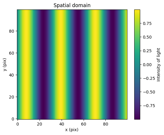
Here we have an image characterized by pixels and intensity. The sinusoidal fringe pattern is a spatial brightness signal with a single “spatial frequency” that can be determined by scanning along a horizontal x-axis perpendicular to the bands.

Now we’ll compute the 2d Fourier transform.

# Take the 2d Fourier transform of the image
fft_sin_tile = fft2(sin_tile)

# Center the freqencies on 0 using fftshift
fft_sin_tile_shifted = fftshift(fft_sin_tile)

# Get the frequencies that fft2 used for the Fourier transform
freqs = fftfreq(n_pixels)

# Center the frequencies on 0 using fftshift
freqs_shifted = fftshift(freqs)

# Plot the original image
fig, ax = plt.subplots(1, 2, figsize=(13, 5))

# Spatial domain plot
im0 = ax[0].imshow(sin_tile, origin="lower", cmap="viridis")
ax[0].set_title("Spatial domain")
ax[0].set_xlabel("x (pix)")
ax[0].set_ylabel("y (pix)")
ax[0].grid("on")
fig.colorbar(im0, ax=ax[0], label="Intensity of light")

# Frequency domain plot
magnitude_spectrum = np.log(np.abs(fft_sin_tile_shifted) + 1)
im1 = ax[1].imshow(
    magnitude_spectrum,
    origin="lower",
    cmap="viridis",
    extent=(freqs_shifted[0], freqs_shifted[-1], freqs_shifted[0], freqs_shifted[-1]),
)
ax[1].set_title("Frequency domain")
ax[1].set_xlabel("Frequency (cycles per pix)")
ax[1].set_ylabel("Frequency (cycles per pix)")
ax[1].grid("on")
fig.colorbar(
    im1, ax=ax[1], label="Log Magnitude of Fourier coefficient for the given frequency"
)

plt.show()

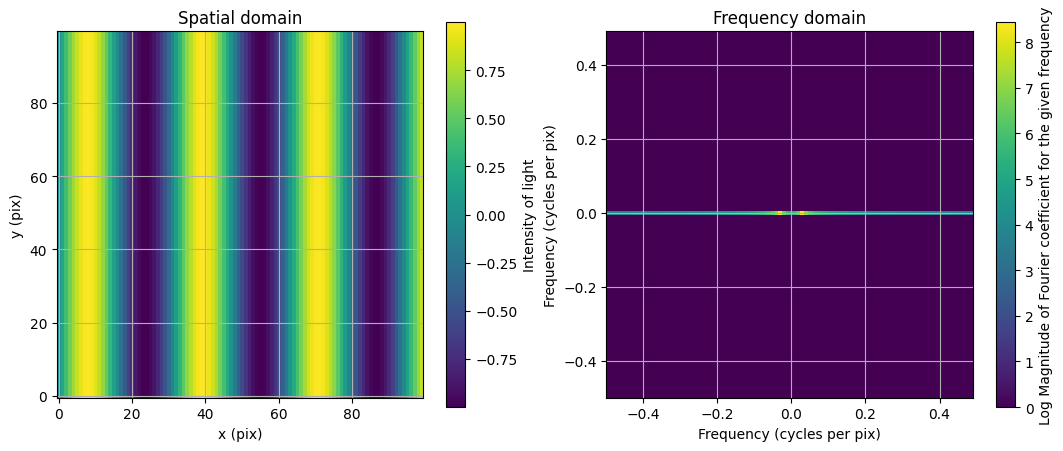
What do we see visually?

Spatial domain

There is a peak approximately every 30 pixels.

Frequency domain

A line of non-zero values along the x-axis which shows us that there are no spatial frequencies that are not strictly horizontal. On that line there are two peaks, which show us where the greatest frequencies are.

Tangent, why the +/- symmetry?

Along the line we have symmetry on the positive and negative axes. This (appears) to be caused by the fact that we have a real-valued function creating our spatial signal, for notation’s sake we’ll refer to \(\sin\) as \(f\) and the Fourier transform as \(F\). The Fourier transform of a real-valued function is by definition Hermitian, meaning that \(F(u, v) = F^*(-u, -v)\). From that property we can establish that the absolute value (magnitude as in the colorbar) of \(F(u,v)\) has the same absolute values as \(F(-u,-v)\). The magnitude of a complex function \(z\) is \(\sqrt{z z^*}\) so $\( |F(u,v)| = \sqrt{F(u,v) F^*(u,v)}\\ \)\( now for the negative values \)\( |F(-u,-v)| = \sqrt{F(-u,-v) F^*(-u,-v)}\\ \)\( \)\( |F(-u,-v)| = \sqrt{F^*(u,v) F(u,v)}\\ \)\( which is equivalent to our expression for \)|F(u,v)|$.

Relating the two

Lets back out the period based on that maximum coefficient.

max_cycles_per_pix_index = np.argmax(np.abs(fft_sin_tile_shifted[50]))
max_cycles_per_pix = np.abs(freqs_shifted[max_cycles_per_pix_index])
print(
    f"Frequency of the maximum Fourier coefficent: {max_cycles_per_pix:.2f} (cycles per pixel)"
)
print(
    f"Period of the spatial domain sinusoid: {1/max_cycles_per_pix:.2f} (pixels per cycle)"
)
print(
    f"Woah, that's pretty close to 5*2pi ({5*2*np.pi:.2f}). Which is the what was used to generate this."
)

Frequency of the maximum Fourier coefficent: 0.03 (cycles per pixel)
Period of the spatial domain sinusoid: 33.33 (pixels per cycle)
Woah, that's pretty close to 5*2pi (31.42). Which is the what was used to generate this.

Recover the spatial domain image from the frequency domain

How well does our frequency domain recreate our spatial domain?

inverted = ifft2(fft_sin_tile).real

# Plot the original image
fig, axs = plt.subplots(ncols=3, figsize=(15, 5))

im0 = axs[0].imshow(sin_tile, origin="lower", cmap="viridis")
axs[0].set_title("Original image")
axs[0].set_xlabel("x (pix)")
axs[0].set_ylabel("y (pix)")
axs[0].grid("on")
# fig.colorbar(im0, ax=axs[0], label="Intensity of light")

im0 = axs[1].imshow(inverted, origin="lower", cmap="viridis")
axs[1].set_title("Reconstructed image")
axs[1].set_xlabel("x (pix)")
axs[1].set_ylabel("y (pix)")
axs[1].grid("on")

# Difference
im0 = axs[2].imshow(
    np.abs(sin_tile - inverted),
    origin="lower",
    cmap="viridis",
    norm=LogNorm(vmin=1e-18, vmax=1e-5),
)
axs[2].set_title("Difference")
axs[2].set_xlabel("x (pix)")
axs[2].set_ylabel("y (pix)")
axs[2].grid("on")
fig.colorbar(im0, ax=axs[2], label="Log difference in intensity of light")
plt.show()

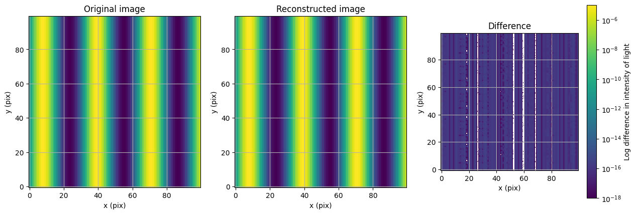
Pretty well!

Moving a 2D image in 1 dimension

Getting back to the translation property of the Fourier transform, let’s shift this along the x-axis. Our equation is \(f(x+a,y) = \int_{-\infty}^{\infty} e^{-i2\pi v_x a} F(v_x,y) e^{i 2 \pi (v_x x)} dv_x\). Let’s break down the terms of that equation.

• \(f(x,y)\) is the function that determines the brightness of a pixel in the image at point \((x, y)\).

• \(a\) is the number of pixels to translate the image in the x direction.

• \(F(v_x,y)\) is the function that determines the strength of a Fourier coefficient at x spatial frequency \(v_x\) (cycles/pixel) and pixel \(y\).

• \(\int_{-\infty}^{\infty} F(v_x,y) e^{i 2 \pi (v_x x)} dv_x\) is the inverse Fourier transform, essentially recreating the original image.

• \(e^{-i2\pi v_x a}\) is the phasor that shifts the original image.

Why is it \((v_x, y)\) and not \((v_x, v_y)\)?

We’re shifting the image in the x direction only, so there is no need to do a full 2d transform, which saves computation. This doesn’t affect the final image at all. But lets test it!

n_pixels = 100
pix_arr = np.arange(0, n_pixels)
sin_vals = np.sin(pix_arr / 5)
sin_tile = np.tile(sin_vals, (n_pixels, 1))

# Take the 1d Fourier transform of the image along the x-axis
fft_sin_tile = fft(sin_tile, axis=1)

# Get the frequencies that fft used for the Fourier transform
freqs = fftfreq(n_pixels)
freqs_shifted = fftshift(freqs)

# Create the phasor
shift_pixels = 15
phasor = np.exp(-2j * np.pi * freqs * shift_pixels)

# Apply the phasor to each row
shifted_fft_sin_tile = fft_sin_tile * phasor

# Reconstruct image
shifted_image = np.real(ifft(shifted_fft_sin_tile, axis=1))

# Plot the original image
fig, ax = plt.subplots(1, 2, figsize=(13, 5))

# Spatial domain plot
im0 = ax[0].imshow(sin_tile, origin="lower", cmap="viridis")
ax[0].set_title("Original image")
ax[0].set_xlabel("x (pix)")
ax[0].set_ylabel("y (pix)")
ax[0].grid("on")
fig.colorbar(im0, ax=ax[0], label="Intensity of light")

# Frequency domain plot
im1 = ax[1].imshow(shifted_image, origin="lower", cmap="viridis")
ax[1].set_title("Shifted image")
ax[1].set_xlabel("x (pix)")
ax[1].set_ylabel("y (pix)")
ax[1].grid("on")
fig.colorbar(im1, ax=ax[1], label="Intensity of light")
fig.savefig("banding.png")
plt.show()

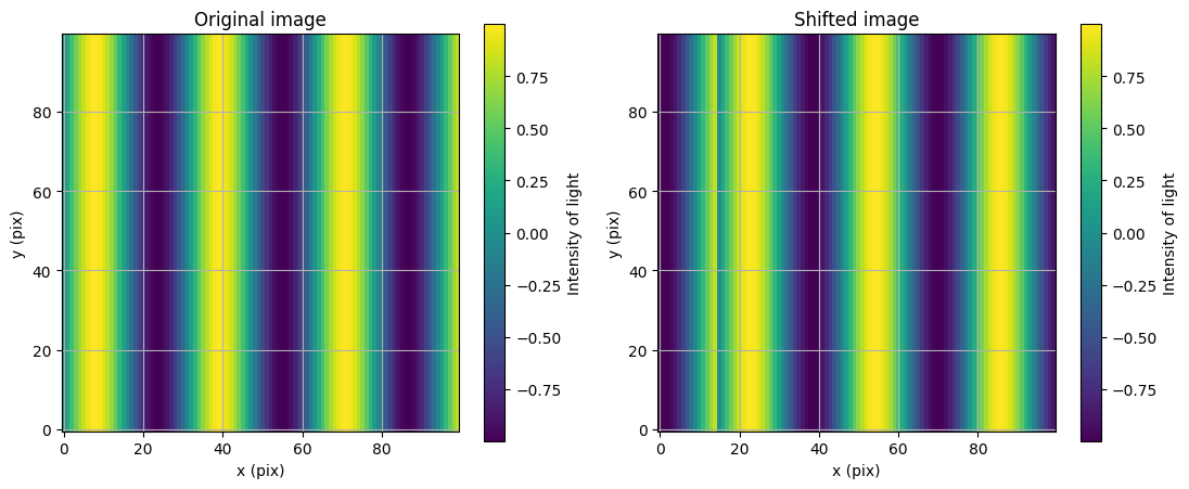
Why is it wrong?

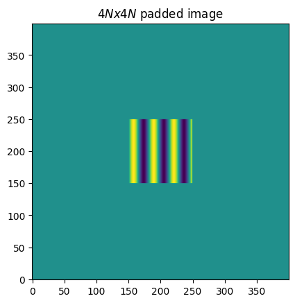
There’s an odd pattern on the left side around pixel 15-20. This is (probably) caused because the FFT does not have the resolution required to handle the low freqency signals. If we were to run that cell without adding the “pix_arr/5” in the sine term it looks fine. Let’s fix this by padding the images with zeros, which expands the range of frequencies that the FFT uses. Looking forward, Larkin et al. recommend padding an NxN image to be 4Nx4N.

padded_image = np.pad(sin_tile, int(1.5 * n_pixels), mode="constant")
plt.imshow(padded_image, origin="lower")
plt.title("$4Nx4N$ padded image")
plt.show()

n_pad = int(1.5 * n_pixels)
img_edge = n_pad + n_pixels

# Pad image with zeros
padded_image = np.pad(sin_tile, n_pad, mode="constant")

# Take the 1d Fourier transform of the image along the x-axis
fft_sin_tile = fft(padded_image, axis=1)

# Get the frequencies that fft used for the Fourier transform
freqs = fftfreq(4 * n_pixels)
freqs_shifted = fftshift(freqs)

# Create the phasor
shift_pixels = 15
phasor = np.exp(-2j * np.pi * freqs * shift_pixels)

# Apply the phasor to each row
shifted_fft_sin_tile = fft_sin_tile * phasor

# Reconstruct image
shifted_image = np.real(ifft(shifted_fft_sin_tile, axis=1))

# Get the unpadded image
unpadded_shifted_image = shifted_image[n_pad:img_edge, n_pad:img_edge]

# Plot the original image
fig, ax = plt.subplots(1, 2, figsize=(13, 5))

# Spatial domain plot
im0 = ax[0].imshow(sin_tile, origin="lower", cmap="viridis")
ax[0].set_title(f"Original image, {sin_tile.shape}")
ax[0].set_xlabel("x (pix)")
ax[0].set_ylabel("y (pix)")
ax[0].grid("on")
fig.colorbar(im0, ax=ax[0], label="Intensity of light")

# Frequency domain plot
im1 = ax[1].imshow(unpadded_shifted_image, origin="lower", cmap="viridis")
ax[1].set_title(f"Shifted image, {unpadded_shifted_image.shape}")
ax[1].set_xlabel("x (pix)")
ax[1].set_ylabel("y (pix)")
ax[1].grid("on")
fig.colorbar(im1, ax=ax[1], label="Intensity of light")
fig.savefig("banding.png")
plt.show()

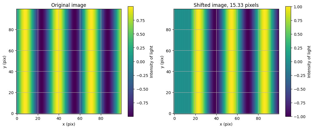
Great! We shited the image without strange effects or adding information that was not in the original image. Let’s set up a function to do it.

def fft_shift(image, shift_pixels):
    n_pixels = image.shape[0]
    n_pad = int(1.5 * n_pixels)
    img_edge = n_pad + n_pixels

    # Pad image with zeros
    padded_image = np.pad(image, n_pad, mode="constant")

    # Take the 1d Fourier transform of the image along the x-axis
    fft_image = fft(padded_image, axis=1)

    # Get the frequencies that fft used for the Fourier transform
    freqs = fftfreq(4 * n_pixels)
    freqs_shifted = fftshift(freqs)

    # Create the phasor
    phasor = np.exp(-2j * np.pi * freqs * shift_pixels)

    # Apply the phasor to each row
    shifted_fft_image = fft_image * phasor

    # Reconstruct image
    shifted_image = np.real(ifft(shifted_fft_image, axis=1))

    # Get the unpadded image
    unpadded_shifted_image = shifted_image[n_pad:img_edge, n_pad:img_edge]
    return unpadded_shifted_image

# Get the unpadded image
unpadded_shifted_image = fft_shift(sin_tile, 15.33)

# Plot the original image
fig, ax = plt.subplots(1, 2, figsize=(13, 5))

# Spatial domain plot
im0 = ax[0].imshow(sin_tile, origin="lower", cmap="viridis")
ax[0].set_title("Original image")
ax[0].set_xlabel("x (pix)")
ax[0].set_ylabel("y (pix)")
ax[0].grid("on")
fig.colorbar(im0, ax=ax[0], label="Intensity of light")

# Frequency domain plot
im1 = ax[1].imshow(unpadded_shifted_image, origin="lower", cmap="viridis")
ax[1].set_title("Shifted image, 15.33 pixels")
ax[1].set_xlabel("x (pix)")
ax[1].set_ylabel("y (pix)")
ax[1].grid("on")
fig.colorbar(im1, ax=ax[1], label="Intensity of light")
fig.savefig("shift.png")
plt.show()

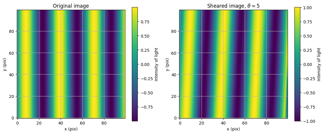
Shearing an image

To do a rotation with FFTs we can break the rotation matrix into three shear matrices. $\( R(\theta) = \begin{pmatrix} \cos\theta & -\sin\theta \\ \sin\theta & \cos\theta \end{pmatrix} = \underbrace{\begin{pmatrix} 1 & -\tan\frac{\theta}{2} \\ 0 & 1 \end{pmatrix}}_{S_x} \underbrace{\begin{pmatrix} 1 & 0 \\ \sin\theta & 1 \end{pmatrix}}_{S_y} \underbrace{\begin{pmatrix} 1 & -\tan\frac{\theta}{2} \\ 0 & 1 \end{pmatrix}}_{S_x} \)$

def frame_center(array):
    """Calculate the center coordinates of an array."""
    return (np.array(array.shape) - 1) / 2

def fft_shear(image, shear_factor, axis):
    """Perform a shear operation in the Fourier domain with proper padding.

    Args:
        image (numpy.ndarray):
            The input image to be sheared.
        shear_factor (float):
            The shear factor.
        axis (int):
            The axis to shear (0 for vertical, 1 for horizontal).

    Returns:
        numpy.ndarray:
            The sheared image with the zero padding removed.
    """
    # Calculate padding size based on the image dimensions
    n_pixels = image.shape[0]
    n_pad = int(1.5 * n_pixels)
    img_edge = n_pad + n_pixels

    # Pad the image with zeros
    padded = np.pad(image, n_pad, mode="constant")

    # Calculate the coordinate array for the padded image
    ori_y, ori_x = padded.shape
    cy, cx = frame_center(padded)
    arr_y, arr_x = np.mgrid[0:ori_y, 0:ori_x]
    coord_array = arr_x - cx if axis == 1 else arr_y - cy

    # Determine the perpendicular axis to the shear direction
    perpendicular_axis = 1 - axis % 2

    # Compute the Fourier frequencies for the dimension perpendicular to the shear axis
    freqs = fftfreq(coord_array.shape[perpendicular_axis])
    freqs = fftshift(freqs)

    # Tile the shifted frequencies to match the dimensions of the padded image
    freqs = np.tile(freqs, (coord_array.shape[axis], 1))

    # Transpose the frequency array if the shear is applied along the horizontal axis
    if axis == 1:
        freqs = freqs.T

    # Shift the padded image to center the zero-frequency component
    padded = fftshift(padded)

    # Apply the Fourier transform along the specified axis
    padded = fft(padded, axis=axis)
    padded = fftshift(padded)

    # Apply the phase shift (shear) in the Fourier domain
    padded = np.exp(-2j * np.pi * shear_factor * freqs * coord_array) * padded

    # Shift back and apply the inverse Fourier transform along the specified axis
    padded = fftshift(padded)
    padded = ifft(padded, axis=axis)
    padded = fftshift(padded)

    # Unpad the image to return to the original size
    image = np.real(padded[n_pad:img_edge, n_pad:img_edge])

    return image

# Get the sheared image
theta = 5
dangle = np.deg2rad(theta)
a = np.tan(dangle / 2)

sheared_image = fft_shear(sin_tile, a, 1)

# Plot the original image
fig, ax = plt.subplots(1, 2, figsize=(13, 5))

# Spatial domain plot
im0 = ax[0].imshow(sin_tile, origin="lower", cmap="viridis")
ax[0].set_title("Original image")
ax[0].set_xlabel("x (pix)")
ax[0].set_ylabel("y (pix)")
ax[0].grid("on")
fig.colorbar(im0, ax=ax[0], label="Intensity of light")

# Frequency domain plot
im1 = ax[1].imshow(sheared_image, origin="lower", cmap="viridis")
ax[1].set_title(f"Sheared image, $\\theta = {theta}$")
ax[1].set_xlabel("x (pix)")
ax[1].set_ylabel("y (pix)")
ax[1].grid("on")
fig.colorbar(im1, ax=ax[1], label="Intensity of light")


fig.savefig("shear.png")
plt.show()

def fft_rotate(image, rot_deg):
    theta = np.deg2rad(rot_deg)
    a = np.tan(theta / 2)
    b = -np.sin(theta)

    # Rotate using three shears
    sx = fft_shear_2(image, a, axis=1)
    sxy = fft_shear_2(sx, b, axis=0)
    sxyx = fft_shear_2(sxy, a, axis=1)
    return sxyx

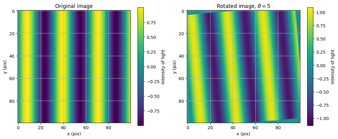
theta = 5
rotated = fft_rotate(sin_tile, 5)

# Plot the original image
fig, ax = plt.subplots(1, 2, figsize=(13, 5))

# Spatial domain plot
im0 = ax[0].imshow(sin_tile, origin="upper", cmap="viridis")
ax[0].set_title("Original image")
ax[0].set_xlabel("x (pix)")
ax[0].set_ylabel("y (pix)")
ax[0].grid("on")
fig.colorbar(im0, ax=ax[0], label="Intensity of light")

# Frequency domain plot
im1 = ax[1].imshow(rotated, origin="upper", cmap="viridis")
ax[1].set_title(f"Rotated image, $\\theta = {theta}$")
ax[1].set_xlabel("x (pix)")
ax[1].set_ylabel("y (pix)")
ax[1].grid("on")
fig.colorbar(im1, ax=ax[1], label="Intensity of light")
fig.savefig("rotate_sin_UL.png")
plt.show()

1D shift

offax_psf_data = pyfits.getdata(Path(yip_path, "offax_psf.fits"))
offax_psf_offsets_list = pyfits.getdata(Path(yip_path, "offax_psf_offset_list.fits"))

psf = offax_psf_data[0]

So let’s implement the equation

\(f(x+a,y) = \int_{-\infty}^{\infty} e^{-i2\pi v_x a} F(v_x,y) e^{i 2 \pi (v_x x)} dv_x\)

Some important conceptual notes before starting:

1. \(x\), \(a\), and \(y\) are in pixels (or whatever the starting array’s units are)

2. \(v_x\) and \(v_y\) are frequency domain transforms of \(x\) and \(y\), giving them units of \(\frac{\text{pixels}}{\text{cycle}}\)

3. At a high level what we are doing is applying a tilt, the Zernicke mode, to the focal plane of our image to change the pupil plane. This works because a tilt in the focal plane corresponds to a change in angle in the pupil plane.

# Number of pixels to shift along the x
a = 80

# The number of x pixels
cols = psf.shape[1]
print(f"Number of x pixels: {cols}")

# Get the sample frequencies that the Discrete Fourier Transform will use (along the x axis)
# Also the frequency bin centers
x_freqs = fftfreq(cols)

# Center the frequences
# e.g. [0, 1, 2, ..., 5, -5, -4, ..., -1] is changed to
# [-5, -4, ..., 0, 1, ..., 5]
v_x = fftshift(x_freqs)

# Example plot of the change
inds = np.arange(cols)
fig, ax = plt.subplots()
ax.plot(inds, x_freqs, label="Original frequencies")
ax.plot(inds, v_x, label="Shifted frequencies")
ax.set_xlabel("Array index")
ax.set_ylabel("Sample frequency, $v_x$")
ax.set_title("Demonstrating fftfreq and the effect of fftshift")
ax.legend()
plt.show()

Number of x pixels: 256

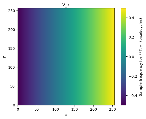
Next, since we are in 2d, we create a tiled version of the sample frequencies so that it applies to all rows of the image. It’s important to note that the equations above have all shown a scalar value, such as \(f(x,y)\), but we are shifting the entire image and not a single pixel so we will work with arrays. Let’s create the array of \(v_x\) values.

V_x = np.tile(v_x, (cols, 1))

fig, ax = plt.subplots()
f = ax.imshow(V_x, origin="lower")
ax.set_xlabel("$x$")
ax.set_ylabel("$y$")
ax.set_title("V_x")
fig.colorbar(f, label="Sample frequency for FFT, $v_x$ (pixel/cycles)")
plt.show()

# This changes the frequency of the tilt
pixels_to_shift = 25

# Create the brightness sinusoid with spatial frequency of pixels_to_shift/
translation_fact = np.exp(-2j * np.pi * (pixels_to_shift * V_x))

phase = np.arctan(translation_fact.imag / translation_fact.real)
intensity = np.abs(translation_fact) ** 2

# Plot the brightness sinusoid
cmap = plt.get_cmap("RdBu")
fig, axes = plt.subplots(ncols=2, figsize=(12, 5))
f = axes[0].imshow(phase, origin="lower", cmap=cmap)
axes[0].set_title("Tilt brightness sinusoid")
fig.colorbar(f, label="Phase (rad)")

# Plot the Fourier transform
axes[1].imshow(np.abs(fft(translation_fact)) ** 2, origin="lower", norm=LogNorm())

plt.show()

# Pixels to shift in X direction
shift_x = 10

# The number of x pixels
rows, cols = psf.shape

# Get the sample frequencies
x = fftfreq(cols)

# This moves the center of the frequency array
sh_x = fftshift(x)

X = np.tile(sh_x, (cols, 1))
translation_fact = np.exp(-2j * np.pi * (shift_x * X))

# Calculate the FFT of the PSF
fft_psf = fft2(psf)

# Multiply the FFT by the translation phasor
shifted_fft_psf = fft_psf * translation_fact

# Get the final PSF
oned_shift = np.abs(ifft2(shifted_fft_psf))


### Plotting
cmap_psf = plt.get_cmap("viridis")
cmap_fft = plt.get_cmap("plasma")
cmap_phasor = plt.get_cmap("cividis")

norm_psf = LogNorm(vmin=psf.min(), vmax=psf.max())
norm_phasor = LogNorm()
norm_fft = LogNorm(vmin=np.abs(fft_psf).min(), vmax=np.abs(fft_psf).max())

base_labels = {"xlabel": "$x$", "ylabel": "$y$"}
fft_labels = {"xlabel": "$x$", "ylabel": "$y$"}

fig, (axes_orig, axes_orig_ffts, axes_phasor, axes_modified_ffts, axes_final) = (
    plt.subplots(ncols=2, nrows=5, figsize=(10, 25))
)

# Show the original information
axes_orig[0].imshow(psf, origin="lower", norm=norm_psf, cmap=cmap_psf)
axes_orig[0].set_title(f"Original PSF, Sum={np.sum(psf):.8e}")
axes_orig[1].imshow(np.abs(fft_psf), origin="lower", norm=norm_fft, cmap=cmap_fft)
axes_orig[1].set_title("Abs(FFT(PSF))")

axes_orig_ffts[0].imshow(
    np.abs(fft_psf.real), origin="lower", norm=norm_fft, cmap=cmap_fft
)
axes_orig_ffts[0].set_title("Real(FFT(PSF))")
axes_orig_ffts[1].imshow(
    np.abs(fft_psf.imag), origin="lower", norm=norm_fft, cmap=cmap_fft
)
axes_orig_ffts[1].set_title("Imag(FFT(PSF))")

axes_phasor[0].imshow(translation_fact.real, origin="lower", cmap=cmap_phasor)
axes_phasor[0].set_title("Real($e^{-i 2 \pi v_x a}$)")
axes_phasor[1].imshow(translation_fact.imag, origin="lower", cmap=cmap_phasor)
axes_phasor[1].set_title("Imag($e^{-i 2 \pi v_x a}$)")

axes_modified_ffts[0].imshow(
    np.abs(shifted_fft_psf.real), origin="lower", norm=norm_fft, cmap=cmap_fft
)
axes_modified_ffts[0].set_title("Real(FFT(PSF)$e^{-i 2 \pi v_x a}$)")
axes_modified_ffts[1].imshow(
    np.abs(shifted_fft_psf.imag), origin="lower", norm=norm_fft, cmap=cmap_fft
)
axes_modified_ffts[1].set_title("Imag(FFT(PSF)*$e^{-i 2 \pi v_x a}$)")

axes_final[0].imshow(
    np.abs(shifted_fft_psf), origin="lower", norm=norm_fft, cmap=cmap_fft
)
axes_final[0].set_title("Abs(FFT(PSF)*$e^{{-i 2 \pi v_x a}}$)")
axes_final[1].imshow(oned_shift, origin="lower", norm=norm_psf, cmap=cmap_psf)
axes_final[1].set_title(f"Shifted PSF, Sum={np.sum(oned_shift):.8e}")


fft_axes = [
    axes_orig[1],
    *axes_orig_ffts,
    *axes_phasor,
    *axes_modified_ffts,
    axes_final[0],
]
for ax in fft_axes:
    ax.set(**fft_labels)
    ax.axvline(cols // 2, ls="--", color="r", alpha=0.5)
    ax.axhline(rows // 2, ls="--", color="r", alpha=0.5)

base_axes = [axes_orig[0], axes_final[1]]
for ax in base_axes:
    ax.set(**base_labels)
    ax.axvline(cols // 2, ls="--", color="r", alpha=0.5)
    ax.axhline(rows // 2, ls="--", color="r", alpha=0.5)

fig.savefig("Shift_example.png", dpi=300, bbox_inches="tight")
# axes_intermediate[1].imshow(np.abs(shifted_fft_psf), origin='lower', norm=norm2)
# axes_intermediate[1].set_title(f"Translated FFT")


# abs_fft = np.abs(fft_psf)

# axes_fft[1].imshow(np.abs(shifted_fft_psf), origin='lower', norm=norm2)
# axes_fft[1].set_title(f"Translated FFT")
# axes_fft[2].imshow(np.abs(shifted_fft_psf-fft_psf), origin='lower', norm=norm2)
# axes_fft[2].set_title(f"Difference")
# plt.show()

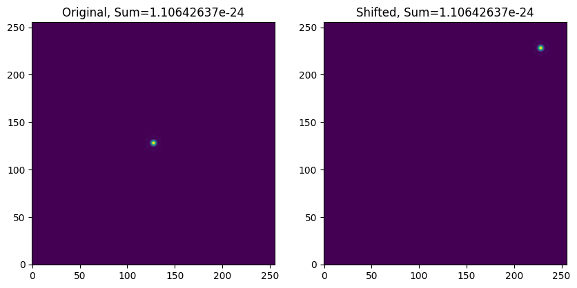
shift_x = 100
shift_y = 100
rows, cols = psf.shape
fft_psf = fft2(psf)
x = fftfreq(cols)
y = fftfreq(rows)
X, Y = np.meshgrid(x, y)

translation_fact = np.exp(-2j * np.pi * (shift_x * X + shift_y * Y))

fft_psf_shifted = fft_psf * translation_fact
translated = ifft2(fft_psf_shifted)
final_psf = np.abs(translated)

fig, axes = plt.subplots(ncols=2, figsize=(10, 5))
axes[0].imshow(psf, origin="lower")
axes[0].set_title(f"Original, Sum={np.sum(psf):.8e}")
axes[1].imshow(final_psf, origin="lower")
axes[1].set_title(f"Shifted, Sum={np.sum(final_psf):.8e}")
plt.show()